
Ocean Acidification in Environmental and Green Chemistry
- Page ID
- 418935
\( \newcommand{\vecs}[1]{\overset { \scriptstyle \rightharpoonup} {\mathbf{#1}} } \)
\( \newcommand{\vecd}[1]{\overset{-\!-\!\rightharpoonup}{\vphantom{a}\smash {#1}}} \)
\( \newcommand{\dsum}{\displaystyle\sum\limits} \)
\( \newcommand{\dint}{\displaystyle\int\limits} \)
\( \newcommand{\dlim}{\displaystyle\lim\limits} \)
\( \newcommand{\id}{\mathrm{id}}\) \( \newcommand{\Span}{\mathrm{span}}\)
( \newcommand{\kernel}{\mathrm{null}\,}\) \( \newcommand{\range}{\mathrm{range}\,}\)
\( \newcommand{\RealPart}{\mathrm{Re}}\) \( \newcommand{\ImaginaryPart}{\mathrm{Im}}\)
\( \newcommand{\Argument}{\mathrm{Arg}}\) \( \newcommand{\norm}[1]{\| #1 \|}\)
\( \newcommand{\inner}[2]{\langle #1, #2 \rangle}\)
\( \newcommand{\Span}{\mathrm{span}}\)
\( \newcommand{\id}{\mathrm{id}}\)
\( \newcommand{\Span}{\mathrm{span}}\)
\( \newcommand{\kernel}{\mathrm{null}\,}\)
\( \newcommand{\range}{\mathrm{range}\,}\)
\( \newcommand{\RealPart}{\mathrm{Re}}\)
\( \newcommand{\ImaginaryPart}{\mathrm{Im}}\)
\( \newcommand{\Argument}{\mathrm{Arg}}\)
\( \newcommand{\norm}[1]{\| #1 \|}\)
\( \newcommand{\inner}[2]{\langle #1, #2 \rangle}\)
\( \newcommand{\Span}{\mathrm{span}}\) \( \newcommand{\AA}{\unicode[.8,0]{x212B}}\)
\( \newcommand{\vectorA}[1]{\vec{#1}} % arrow\)
\( \newcommand{\vectorAt}[1]{\vec{\text{#1}}} % arrow\)
\( \newcommand{\vectorB}[1]{\overset { \scriptstyle \rightharpoonup} {\mathbf{#1}} } \)
\( \newcommand{\vectorC}[1]{\textbf{#1}} \)
\( \newcommand{\vectorD}[1]{\overrightarrow{#1}} \)
\( \newcommand{\vectorDt}[1]{\overrightarrow{\text{#1}}} \)
\( \newcommand{\vectE}[1]{\overset{-\!-\!\rightharpoonup}{\vphantom{a}\smash{\mathbf {#1}}}} \)
\( \newcommand{\vecs}[1]{\overset { \scriptstyle \rightharpoonup} {\mathbf{#1}} } \)
\(\newcommand{\longvect}{\overrightarrow}\)
\( \newcommand{\vecd}[1]{\overset{-\!-\!\rightharpoonup}{\vphantom{a}\smash {#1}}} \)
\(\newcommand{\avec}{\mathbf a}\) \(\newcommand{\bvec}{\mathbf b}\) \(\newcommand{\cvec}{\mathbf c}\) \(\newcommand{\dvec}{\mathbf d}\) \(\newcommand{\dtil}{\widetilde{\mathbf d}}\) \(\newcommand{\evec}{\mathbf e}\) \(\newcommand{\fvec}{\mathbf f}\) \(\newcommand{\nvec}{\mathbf n}\) \(\newcommand{\pvec}{\mathbf p}\) \(\newcommand{\qvec}{\mathbf q}\) \(\newcommand{\svec}{\mathbf s}\) \(\newcommand{\tvec}{\mathbf t}\) \(\newcommand{\uvec}{\mathbf u}\) \(\newcommand{\vvec}{\mathbf v}\) \(\newcommand{\wvec}{\mathbf w}\) \(\newcommand{\xvec}{\mathbf x}\) \(\newcommand{\yvec}{\mathbf y}\) \(\newcommand{\zvec}{\mathbf z}\) \(\newcommand{\rvec}{\mathbf r}\) \(\newcommand{\mvec}{\mathbf m}\) \(\newcommand{\zerovec}{\mathbf 0}\) \(\newcommand{\onevec}{\mathbf 1}\) \(\newcommand{\real}{\mathbb R}\) \(\newcommand{\twovec}[2]{\left[\begin{array}{r}#1 \\ #2 \end{array}\right]}\) \(\newcommand{\ctwovec}[2]{\left[\begin{array}{c}#1 \\ #2 \end{array}\right]}\) \(\newcommand{\threevec}[3]{\left[\begin{array}{r}#1 \\ #2 \\ #3 \end{array}\right]}\) \(\newcommand{\cthreevec}[3]{\left[\begin{array}{c}#1 \\ #2 \\ #3 \end{array}\right]}\) \(\newcommand{\fourvec}[4]{\left[\begin{array}{r}#1 \\ #2 \\ #3 \\ #4 \end{array}\right]}\) \(\newcommand{\cfourvec}[4]{\left[\begin{array}{c}#1 \\ #2 \\ #3 \\ #4 \end{array}\right]}\) \(\newcommand{\fivevec}[5]{\left[\begin{array}{r}#1 \\ #2 \\ #3 \\ #4 \\ #5 \\ \end{array}\right]}\) \(\newcommand{\cfivevec}[5]{\left[\begin{array}{c}#1 \\ #2 \\ #3 \\ #4 \\ #5 \\ \end{array}\right]}\) \(\newcommand{\mattwo}[4]{\left[\begin{array}{rr}#1 \amp #2 \\ #3 \amp #4 \\ \end{array}\right]}\) \(\newcommand{\laspan}[1]{\text{Span}\{#1\}}\) \(\newcommand{\bcal}{\cal B}\) \(\newcommand{\ccal}{\cal C}\) \(\newcommand{\scal}{\cal S}\) \(\newcommand{\wcal}{\cal W}\) \(\newcommand{\ecal}{\cal E}\) \(\newcommand{\coords}[2]{\left\{#1\right\}_{#2}}\) \(\newcommand{\gray}[1]{\color{gray}{#1}}\) \(\newcommand{\lgray}[1]{\color{lightgray}{#1}}\) \(\newcommand{\rank}{\operatorname{rank}}\) \(\newcommand{\row}{\text{Row}}\) \(\newcommand{\col}{\text{Col}}\) \(\renewcommand{\row}{\text{Row}}\) \(\newcommand{\nul}{\text{Nul}}\) \(\newcommand{\var}{\text{Var}}\) \(\newcommand{\corr}{\text{corr}}\) \(\newcommand{\len}[1]{\left|#1\right|}\) \(\newcommand{\bbar}{\overline{\bvec}}\) \(\newcommand{\bhat}{\widehat{\bvec}}\) \(\newcommand{\bperp}{\bvec^\perp}\) \(\newcommand{\xhat}{\widehat{\xvec}}\) \(\newcommand{\vhat}{\widehat{\vvec}}\) \(\newcommand{\uhat}{\widehat{\uvec}}\) \(\newcommand{\what}{\widehat{\wvec}}\) \(\newcommand{\Sighat}{\widehat{\Sigma}}\) \(\newcommand{\lt}{<}\) \(\newcommand{\gt}{>}\) \(\newcommand{\amp}{&}\) \(\definecolor{fillinmathshade}{gray}{0.9}\)
-
V.D.3.a. Categorizing reactions in terms of acid–base chemistry, particularly in water, is important
-
V.D.3.b. Categorizing acid–base reactions can be facilitated by a basic understanding of acid–base strength.
-
V.D.3.c. The definition of an acid as a proton donor and a base as a proton acceptor is a key concept of acid–base chemistry.
-
VIII.G.1.a. Acid–base chemistry, particularly in water, forms an important example of equilibrium systems. Conceptual and quantitative understanding of this form of equilibrium system is important.
-
VII.G.1.b. The laboratory technique of titration serves as a key example for acid– base chemistry; interpretation of titration curves, both conceptually and quantitatively, is an important tool for chemists.
-
VIII.G.1.c. pH is used in quantitative descriptions of acid–base chemistry.
-
VIII.G.2.a. Weak acid–base systems are capable of forming buffer systems that tend to resist changes in the pH of the system.
-
VIII.G.2.b. Conceptual and quantitative understanding of buffers is important.
-
X.D. Quantitative reasoning within chemistry is often visualized and interpreted graphically.
-
X.E.1. Rearrangement of common mathematical expressions can either isolate variables or identify relationships that enhance understanding of the system being described.
Environmental and green chemistry focuses on the effects of human behavior on our environment and implementing measures to minimize harm to our planet. The advent of the industrial revolution has caused an increase in the concentration of \(CO_2\) in the atmosphere. The heat trapped by the greenhouse gases has led to an increase in global temperatures, commonly known as global warming. However, a critical and lesser reported change is also affecting the world’s oceans. As the ocean continues to absorb the \(CO_2\) emissions, the concentration of hydrogen ions have increased, lowering the pH of the ocean in a phenomenon known as ocean acidification. This is very harmful for marine ecosystems, as it reduces the amount of free carbonate ions available for shell and skeleton building organisms, such as pteropods or corals, to build their homes (more on this will be explained later). The decrease in pH also forces species to either adapt to a pH outside of their comfortable range or become extinct, such as inducing zooxanthellae to flee from the polyps of corals in a phenomenon known as coral bleaching[1]. To provide context, we will explain the chemistry behind ocean acidification, and how we can use the ocean’s buffer system, the Henderson-Hasselbach equation, and ionic ratios to explain how higher levels of \(CO_2\) disrupt the equilibrium of the ocean.
pH Explained
pH is a measure of the logarithmic measure of the concentration of hydrogen ions in a solution, defined as the \(-\log_{10}([H^+])\). The pH scale runs from 0 to 14, with 7 being a neutral pH. Anything higher than 7 is basic (or alkaline) and anything lower than 7 is acidic. A negative in the logarithmic scale means it is an inverse function, as \(-\log_{10}(x) = \log(1/x)\). Oceans have recorded a drop in pH of approximately 0.1 since the Industrial Revolution, and is currently at a pH of around 8.3. While this drop may not seem significant, you must remember the scale is logarithmic, so the magnitude of increase in \([H^+]\) is exponentially greater. These aqueous \([H^+]\) ions bond with \(H_2O\) molecules to form \(H_3O^+\), the hydronium ion, so more accurately the pH would be \(-\log_{10}([H_3O^+])\). Imagine the ocean as a very large human body, there are processes inside the body to maintain health and ensure everything is in working order. If our pH range drops 0.1, this can cause significant damage to the cells of our bodies as it tries to establish equilibrium. Likewise, many species will be subjected to conditions outside of their normal pH range, or find it harder to find free carbonate to build their exoskeletons.
Measuring pH
pH can be measured in a multitude of ways. This section will discuss some of the ways scientists today monitor the pH of the world’s oceans.
One method of measurement is using an ion sensitive field effect transistor (ISFET). This device can measure the pH by placing a single drop of an ocean sample onto a silicon chip sensor and based on the current running through the transistor, it can determine the concentration of \([H^+]\) ions present. ISFETs are attached to ships, stationary buoys or floats and lowered into the ocean for periods of time, so scientists can maintain continuous logs of ocean pH[2].
Another method is using pH reactive dyes or pH paper. When these substances react with \([H^+]\) ions, they will change colors depending on whether the solution is more acidic or basic. Each pH indicator has its own effective range, so it is important to consider the estimated pH you are measuring before choosing one. Common pH indicators are phenolphthalein (range pH 8.2 to 10.0; colorless to pink), bromothymol blue (range pH 6.0 to 7.6; yellow to blue), and litmus (range pH 4.5 to 8.3; red to blue).
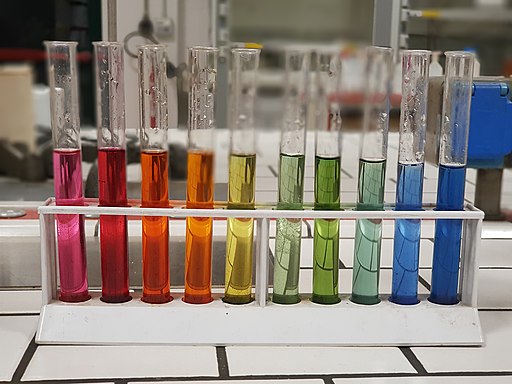.jpg?revision=1)
Figure \(\PageIndex{1}\): pH Scale Indicators. (CC BY 4.0; via Wikimedia Commons)
Buffers
A buffer is a solution that is able to resist pH changes upon addition of an acid or base. This is due to the fact that the buffer has both the conjugate acid and base pair present. Buffers have a buffer capacity and a buffer range. Buffer capacity is the amount of strong acid/base that must be added before the pH changes significantly, while buffer range is the constant pH range that a buffer maintains when it neutralizes additional acid/base[3]. This relationship can be best shown through a titration curve.

Figure \(\PageIndex{2}\): General Titration Curve of a Weak Acid and Strong Base. (Created by Sarah Lin)
The pH of a buffer can be estimated using the Henderson-Hasselbach equation.
Henderson-Hasselbach Equation
The Henderson-Hasselbach equation shows the relationship between the pH and acid dissociation constant of an aqueous solution of an acid[4]. The equation is shown below:
\[p H=p K_a+\log _{10}\left(\frac{[\text { conjugate base }]}{[\text { weak acid }]}\right) \nonumber\]
Below is the derivation for this relationship, using the hypothetical weak acid, HA:
This represents the acid in water.
\[\mathrm{HA}_{(a q)}+\mathrm{H}_2 \mathrm{O} \underset{(l)}{ } \leftrightharpoons A_{(a q)}^{-}+\mathrm{H}_3 \mathrm{O}_{(a q)}^{+}\]
From this, we can derive the acid dissociation constant expression.
\[K_a=\frac{\left[A^{-}\right]\left[H_3 O^{+}\right]}{[H A]}\]
Multiply both sides by \([{HA}]\)
\[K_a[H A]=\left[A^{-}\right]\left[H_3 O^{+}\right]\]
Divide both sides by \([{A}^-]\)
\[\frac{K_a[H A]}{\left[A^{-}\right]}=\left[H_3 O^{+}\right]\]
Flip the equation and take the log
\[\log _{10}\left[H_3 O^{+}\right]=\log _{10}\left[K_a\right]+\log _{10} \frac{[H A]}{\left[A^{-}\right]}\]
Multiply both sides by -1
\[-\log _{10}\left[H_3 O^{+}\right]=-\log _{10}\left[K_a\right]-\log _{10} \frac{[H A]}{\left[A^{-}\right]}\]
Replace -log with p
\[p H=p K_a-\log _{10} \frac{[H A]}{\left[A^{-}\right]}\]
Use property that \(n \times \log_{10}(x)=\log_{10}({x}^{n})\)
\[p H=p K_a+\log _{10} \frac{\left[A^{-}\right]}{[H A]}\]
The ocean has a carbonate/hydrogen carbonate buffer system in the series of equilibrium reactions. Shown below is a simplified series of reactions:
\[\mathrm{CO}_2(a q)+\mathrm{H}_2 \mathrm{O}(l) \rightleftharpoons \mathrm{H}_2 \mathrm{CO}_3(a q) \rightleftharpoons H^{+}(a q)+\mathrm{HCO}_3{ }^{-}(a q) \nonumber\]
We can see how \(CO_2\) induces the dissociation of \(H^+\) ions by the formation and dissociation of carbonic acid into bicarbonate and hydrogen ions, and the further dissociation of bicarbonate into carbonate and hydrogen ions[5]. The majority of the hydrogen ions produced in the dissociation of carbonic acid contribute to lowering the pH of the ocean. For example, we can incorporate the ratios of hydrogen carbonate and carbonic acid to estimate the pH of the ocean in the sample problem below.
If the ratio of the concentrations of \([{HCO}_3{ }^-]\) to \([{H}_{2}{CO}_{3}]\) is 90:1, Calculate the pH of the ocean given that the \({K}_{a}\), or acid dissociation constant of carbonic acid \({H}_{2}{CO}_{3}\) is \({4.5} \times {10}^{-7}\)
(Note, ratio is not representative of the actual concentrations of ions, as equilibrium systems in the ocean are much more complex).
Solution
Calculate the pKa
\[-\log \left(K_a\right)=-\log \left(4.5 \times 10^{-7}\right) \approx 6.3468\]
Use the Henderson-Hasselbach equation
\[p H=p K_a+\log _{10}\left(\frac{[\text { conjugate base }]}{[\text { weak acid }]}\right)\]
Plug in values and solve
\[p H=p K_a+\log _{10}\left(\frac{\left[\mathrm{HCO}_3^{-}\right]}{\left[\mathrm{H}_2 \mathrm{CO}_3\right]}\right)\]
\[p H=6.3468+\log _{10}(90)\]
\[p H \approx 8.3010\]
Polyprotic Acids
The example above sacrifices accuracy for the sake of simplicity, assuming that \(H_2{CO}_3\) is a monoprotic acid. \(H_2{CO}_3\) contains two hydrogens, which means it is actually capable of donating two \(H^+\) ions to a solution (5). These types of acids are called polyprotic acids. \(H^+\) ions are lost in stages with the first proton being the most readily lost. Each of the dissociations of \(H_2{CO}_3\) in water can be represented as shown below:
\[\mathrm{H}_2 \mathrm{CO}_3(a q)+\mathrm{H}_2 \mathrm{O}(l) \rightleftharpoons \mathrm{H}^{+}(a q)+\mathrm{HCO}_3{ }^{-}(a q) \quad K_{a 1}=4.5 \times 10^{-7}\]
\[\mathrm{HCO}_3{ }^{-}(a q)+\mathrm{H}_2 \mathrm{O}(l) \rightleftharpoons \mathrm{H}^{+}(a q)+\mathrm{CO}_3{ }^{2-}(a q) \quad K_{a 2}=4.7 \times 10^{-11}\]
For all polyprotic acids, \(\mathrm{K}_{\mathrm{a} 1}>\mathrm{K}_{\mathrm{a} 2}>\mathrm{K}_{\mathrm{a} 3}\)
For \(\mathrm{H_2{CO}_3}\), using the dissociation reactions, we can determine the \(K_{a 1}\) and \(K_{a 2}\) expressions:
\[K_{a 1}=\frac{\left[\mathrm{H}^{+}\right]\left[\mathrm{HCO}_3{ }^{-}\right]}{\left[\mathrm{H}_2 \mathrm{CO}_3\right]}\]
\[K_{a 2}=\frac{\left[\mathrm{H}^{+}\right]\left[\mathrm{CO}_3{ }^{2-}\right]}{\left[\mathrm{HCO}_3{ }^{-}\right]}\]

Figure \(\PageIndex{3}\): Titration Curve of Carbonic Acid. (CC BY-SA; via Wikimedia Commons)
Using these polyprotic properties, we can more accurately calculate the change in carbonate from a 0.1 decrease in pH. Below is an example problem of how ocean acidification reduces the amount of free carbonate for organisms.
Since the Industrial Revolution and the release of \({CO}_{2}\) emissions, there has been a drop in ocean pH from 8.2 to 8.1. How does this affect the fraction of carbonate in the ocean?
Solution
Determine the equilibrium expressions for each stage of dissociation
\[\mathrm{CO}_{2}(\mathrm{aq})+\mathrm{H}_{2} \mathrm{O}(l) \rightleftharpoons \mathrm{H}_{2} \mathrm{CO}_{3}(a q)\]
\[\mathrm{H}_{2} \mathrm{CO}_{3}(\mathrm{aq}) \rightleftharpoons \mathrm{H}^{+}(\mathrm{aq})+\mathrm{HCO}_3{ }^{-}(\mathrm{aq}) \quad \mathrm{K}_{a \, \mathrm{H}_{2} \mathrm{CO}_{3}}=4.5 \times 10^{-7}=\mathrm{K}_{a1}\]
\[\mathrm{HCO}_3{ }^{-}(\mathrm{aq}) \rightleftharpoons \mathrm{H}^{+}(\mathrm{aq})+\mathrm{CO}_3{ }^{-}(\mathrm{aq}) \quad \mathrm{K}_{a \, \mathrm{HCO}_3{ }^-}=4.7 \times 10^{-11}=\mathrm{K}_{a 2}\]
Write the \({K}_{a}\) expressions for each equilibrium
\[K_{a 1}=\frac{\left[\mathrm{HCO}_3{ }^{-}\right]\left[\mathrm{H}^{+}\right]}{\left[\mathrm{H}_{2} \mathrm{CO}_{3}\right]} \quad K_{a 2}=\frac{\left[\mathrm{CO}_3{ }^{2-}\right]\left[\mathrm{H}^{+}\right]}{\left[\mathrm{HCO}_3{ }^{-}\right]}\]
The fraction of carbonate present can be defined as the equilibrium concentration of carbonate divided by the sum of equilibrium concentrations of all compounds present in the solution ( \(\mathrm{H_{2}{CO}_{3}}\), \(\mathrm{HCO}_3{ }^-\), \(\mathrm{CO}_3{ }^{2-}\) )
\[\operatorname{fraction}\left(\mathrm{CO}_{3}{ }^{2-}\right)=\frac{\left[\mathrm{CO}_{3}{ }^{2-}\right]_{e q}}{\left[\mathrm{H}_{2} \mathrm{CO}_{3}\right]_{e q}+\left[\mathrm{HCO}_{3}{ }^{-}\right]_{e q}+\left[\mathrm{CO}_{3}{ }^{2-}\right]_{e q}}\]
Rearrange each of the \({K}_{a}\) expressions so they are in terms of \(\mathrm{HCO}_3{ }^-\)
\[\left[\mathrm{H}_{2} \mathrm{CO}_{3}\right]=\frac{\left[\mathrm{HCO}_3{ }^{-}\right]\left[\mathrm{H}^{+}\right]}{\mathrm{K}_{a 1}} \quad\left[\mathrm{CO}_3{ }^{2-}\right]=\frac{\mathrm{K}_{a 2}\left[\mathrm{HCO}_3{ }^{-}\right]}{\left[\mathrm{H}^{+}\right]}\]
Plug in and simplify the expression
\[f=\frac{\frac{\mathrm{K}_{a2}\left[\mathrm{HCO}_3{ }^{-}\right]}{\left[\mathrm{H}^{+}\right]}}{\frac{\left[\mathrm{HCO}_3{ }^{-}\right]\left[\mathrm{H}^{+}\right]}{\mathrm{K}_{a1}}+\left[\mathrm{HCO}_3{ }^-\right]+\frac{\mathrm{K}_{a2}\left[\mathrm{HCO}_3{ }^{-}\right]}{\left[\mathrm{H}^{+}\right]}}=\frac{\frac{\mathrm{K}_{a2}}{\left[\mathrm{H}^{+}\right]}}{\frac{\left[\mathrm{H}^{+}\right]}{\mathrm{K}_{a1}}+1+\frac{K _{a2}}{\left[\mathrm{H}^{+}\right]}}\]
At pH of 8.2: \([{H}^+]=10^{-8.2}=6.31 \times 10^{-9}\)
\[f=\frac{\frac{4.7 \times 10^{-11}}{6.31 \times 10^{-9}}}{\frac{6.31 \times 10^{-9}}{4.5 \times 10^{-7}}+1+\frac{4.7 \times 10^{-11}}{6.31 \times 10^{-9}}}=0.00730\]
At pH of 8.1: \([{H}^+]=10^{-8.1}=7.9433 \times 10^{-9}\)
\[f=\frac{\frac{4.7 \times 10^{-11}}{7.9433 \times 10^{-9}}}{\frac{7.9433 \times 10^{-9}}{4.5 \times 10^{-7}}+1+\frac{4.7 \times 10^{-11}}{7.9433 \times 10^{-9}}}=0.00578\]
Subtract the calculated values \(0.00730-0.00578=0.00152\). Fraction of carbonate decreases by approximately \(0.00152\).
As you can see, even a drop of 0.1 in pH can significantly affect the fraction of carbonate in the ocean. This affects the availability of free carbonate in the ocean for organisms such as mollusks to build shells, and for corals to build carbonate skeletons[6].
References
- ACS Climate Science Working Group. Ocean Chemistry. ACS Climate Science Toolkit. https://www.acs.org/content/acs/en/c...chemistry.html (accessed 2022-10-28).
-
Ocean Acidification. National Oceanic and Atmospheric Administration, 2020. https://www.noaa.gov/education/resou...-acidification (accessed 2022-10-28).
-
10.5: Buffers. LibreTexts, 2022. https://chem.libretexts.org/Bookshel....05%3A_Buffers (accessed 2022-10-28).
-
Gunawardena, G. Henderson-Hasselbach Equation. LibreTexts, 2022. https://chem.libretexts.org/Ancillar...lbach_Equation (accessed 2022-10-28).
-
Graduate School of Education (SPICE Program). Buffers 4: Researching Ocean Buffering (Fact Sheet). The University of Western Australia, 2011. https://www.uwa.edu.au/study/-/media...-buffering.pdf (accessed 2022-10-28).
-
Barker, S.; Ridgwell, A. Ocean Acidification. Nature Education Knowledge Project, 2012. https://www.nature.com/scitable/know...%25%20of%20DIC (accessed 2022-10-28).