
Determining Climate Change with Isotopes in Environmental and Green Chemistry
- Page ID
- 418912
\( \newcommand{\vecs}[1]{\overset { \scriptstyle \rightharpoonup} {\mathbf{#1}} } \)
\( \newcommand{\vecd}[1]{\overset{-\!-\!\rightharpoonup}{\vphantom{a}\smash {#1}}} \)
\( \newcommand{\dsum}{\displaystyle\sum\limits} \)
\( \newcommand{\dint}{\displaystyle\int\limits} \)
\( \newcommand{\dlim}{\displaystyle\lim\limits} \)
\( \newcommand{\id}{\mathrm{id}}\) \( \newcommand{\Span}{\mathrm{span}}\)
( \newcommand{\kernel}{\mathrm{null}\,}\) \( \newcommand{\range}{\mathrm{range}\,}\)
\( \newcommand{\RealPart}{\mathrm{Re}}\) \( \newcommand{\ImaginaryPart}{\mathrm{Im}}\)
\( \newcommand{\Argument}{\mathrm{Arg}}\) \( \newcommand{\norm}[1]{\| #1 \|}\)
\( \newcommand{\inner}[2]{\langle #1, #2 \rangle}\)
\( \newcommand{\Span}{\mathrm{span}}\)
\( \newcommand{\id}{\mathrm{id}}\)
\( \newcommand{\Span}{\mathrm{span}}\)
\( \newcommand{\kernel}{\mathrm{null}\,}\)
\( \newcommand{\range}{\mathrm{range}\,}\)
\( \newcommand{\RealPart}{\mathrm{Re}}\)
\( \newcommand{\ImaginaryPart}{\mathrm{Im}}\)
\( \newcommand{\Argument}{\mathrm{Arg}}\)
\( \newcommand{\norm}[1]{\| #1 \|}\)
\( \newcommand{\inner}[2]{\langle #1, #2 \rangle}\)
\( \newcommand{\Span}{\mathrm{span}}\) \( \newcommand{\AA}{\unicode[.8,0]{x212B}}\)
\( \newcommand{\vectorA}[1]{\vec{#1}} % arrow\)
\( \newcommand{\vectorAt}[1]{\vec{\text{#1}}} % arrow\)
\( \newcommand{\vectorB}[1]{\overset { \scriptstyle \rightharpoonup} {\mathbf{#1}} } \)
\( \newcommand{\vectorC}[1]{\textbf{#1}} \)
\( \newcommand{\vectorD}[1]{\overrightarrow{#1}} \)
\( \newcommand{\vectorDt}[1]{\overrightarrow{\text{#1}}} \)
\( \newcommand{\vectE}[1]{\overset{-\!-\!\rightharpoonup}{\vphantom{a}\smash{\mathbf {#1}}}} \)
\( \newcommand{\vecs}[1]{\overset { \scriptstyle \rightharpoonup} {\mathbf{#1}} } \)
\(\newcommand{\longvect}{\overrightarrow}\)
\( \newcommand{\vecd}[1]{\overset{-\!-\!\rightharpoonup}{\vphantom{a}\smash {#1}}} \)
\(\newcommand{\avec}{\mathbf a}\) \(\newcommand{\bvec}{\mathbf b}\) \(\newcommand{\cvec}{\mathbf c}\) \(\newcommand{\dvec}{\mathbf d}\) \(\newcommand{\dtil}{\widetilde{\mathbf d}}\) \(\newcommand{\evec}{\mathbf e}\) \(\newcommand{\fvec}{\mathbf f}\) \(\newcommand{\nvec}{\mathbf n}\) \(\newcommand{\pvec}{\mathbf p}\) \(\newcommand{\qvec}{\mathbf q}\) \(\newcommand{\svec}{\mathbf s}\) \(\newcommand{\tvec}{\mathbf t}\) \(\newcommand{\uvec}{\mathbf u}\) \(\newcommand{\vvec}{\mathbf v}\) \(\newcommand{\wvec}{\mathbf w}\) \(\newcommand{\xvec}{\mathbf x}\) \(\newcommand{\yvec}{\mathbf y}\) \(\newcommand{\zvec}{\mathbf z}\) \(\newcommand{\rvec}{\mathbf r}\) \(\newcommand{\mvec}{\mathbf m}\) \(\newcommand{\zerovec}{\mathbf 0}\) \(\newcommand{\onevec}{\mathbf 1}\) \(\newcommand{\real}{\mathbb R}\) \(\newcommand{\twovec}[2]{\left[\begin{array}{r}#1 \\ #2 \end{array}\right]}\) \(\newcommand{\ctwovec}[2]{\left[\begin{array}{c}#1 \\ #2 \end{array}\right]}\) \(\newcommand{\threevec}[3]{\left[\begin{array}{r}#1 \\ #2 \\ #3 \end{array}\right]}\) \(\newcommand{\cthreevec}[3]{\left[\begin{array}{c}#1 \\ #2 \\ #3 \end{array}\right]}\) \(\newcommand{\fourvec}[4]{\left[\begin{array}{r}#1 \\ #2 \\ #3 \\ #4 \end{array}\right]}\) \(\newcommand{\cfourvec}[4]{\left[\begin{array}{c}#1 \\ #2 \\ #3 \\ #4 \end{array}\right]}\) \(\newcommand{\fivevec}[5]{\left[\begin{array}{r}#1 \\ #2 \\ #3 \\ #4 \\ #5 \\ \end{array}\right]}\) \(\newcommand{\cfivevec}[5]{\left[\begin{array}{c}#1 \\ #2 \\ #3 \\ #4 \\ #5 \\ \end{array}\right]}\) \(\newcommand{\mattwo}[4]{\left[\begin{array}{rr}#1 \amp #2 \\ #3 \amp #4 \\ \end{array}\right]}\) \(\newcommand{\laspan}[1]{\text{Span}\{#1\}}\) \(\newcommand{\bcal}{\cal B}\) \(\newcommand{\ccal}{\cal C}\) \(\newcommand{\scal}{\cal S}\) \(\newcommand{\wcal}{\cal W}\) \(\newcommand{\ecal}{\cal E}\) \(\newcommand{\coords}[2]{\left\{#1\right\}_{#2}}\) \(\newcommand{\gray}[1]{\color{gray}{#1}}\) \(\newcommand{\lgray}[1]{\color{lightgray}{#1}}\) \(\newcommand{\rank}{\operatorname{rank}}\) \(\newcommand{\row}{\text{Row}}\) \(\newcommand{\col}{\text{Col}}\) \(\renewcommand{\row}{\text{Row}}\) \(\newcommand{\nul}{\text{Nul}}\) \(\newcommand{\var}{\text{Var}}\) \(\newcommand{\corr}{\text{corr}}\) \(\newcommand{\len}[1]{\left|#1\right|}\) \(\newcommand{\bbar}{\overline{\bvec}}\) \(\newcommand{\bhat}{\widehat{\bvec}}\) \(\newcommand{\bperp}{\bvec^\perp}\) \(\newcommand{\xhat}{\widehat{\xvec}}\) \(\newcommand{\vhat}{\widehat{\vvec}}\) \(\newcommand{\uhat}{\widehat{\uvec}}\) \(\newcommand{\what}{\widehat{\wvec}}\) \(\newcommand{\Sighat}{\widehat{\Sigma}}\) \(\newcommand{\lt}{<}\) \(\newcommand{\gt}{>}\) \(\newcommand{\amp}{&}\) \(\definecolor{fillinmathshade}{gray}{0.9}\)I. A. 2. b. Atoms of one element have the same number of protons but can have differing numbers of neutrons. These are called isotopes.
I. A. 2. d. The isotopic abundance of any given element is not a constant of nature, and may vary depending on the origin of the sample being studied.
IV. A. 2. Properties that depend on intermolecular forces include phase, vapor pressure, surface tension, etc.
IX. E. 4. a. Mass spectrometry data can be used to illustrate the existence of isotopes of an element and the importance of isotopic abundances.
Climate Change
In recent years, the rise of climate change has drastically been at the forefront of environmental concern, associated with rising average global temperatures and detriment to ecosystems all around the world. The study of climate change revolves around key factors that may lead to these dramatically changing communities and this can be done through tracking changes in the history of certain area’s average temperatures. Using chemistry, specifically isotopes, to track the progression of climate change over past decades can be this link to our full understanding of the development of these rising temperatures. By analyzing the typically observed temperature fluctuations over history, abnormal phenomena are identifiable.
Isotopes
Although the identity of an atom is dependent on its number of protons, and this value remains constant, the number of neutrons can vary within species of the same element. Isotopes are forms of an element that have the same amount of protons, but differ in their number of neutrons. As a result, not all species of an element have the same mass; therefore, the average atomic mass of an element represented on the periodic table is never a whole number, taking into account the various isotopes of the same element.1
The isotopic abundance of an element is the relative proportion of isotopes for a given element. The isotopic abundance varies as some isotopes are more common than others. Typically, these proportions are represented as percentages and their sum must be 100%.1 A mass spectrometer allows researchers to determine the relative abundance of isotopes in a sample. This device produces data regarding the relative abundance of isotopes, or the isotopic abundance of an element and can be used to calculate average atomic mass using the formula below.1
\[ \text { Average Atomic Mass } \left.=\sum \text { (relative abundance of isotope } n\right) \times(\text { mass of isotope } n) \nonumber\]
Isotopes of Oxygen
One atom that is known for having distinct isotopes is oxygen: Oxygen-16, Oxygen-17, and Oxygen-18. Oxygen has 8 protons and 8 electrons with a mass number really close to 16.00, so in nature, it most commonly exists as Oxygen-16 with 8 neutrons. However, Oxygen-18 is found in small quantities (about 1 in 500 atoms), but Oxygen-17 has an even lower isotopic abundance and usually is not taken into consideration. Because Oxygen-18 has two more neutrons than Oxygen-16, Oxygen-18 has a greater mass and is a bulkier atom, as shown in the image below.2

Figure 1. Atomic level diagram of Oxygen-16 and Oxygen-18. Source: NASA Earth Observatory.2
Using the results of the mass spectroscopy of a sample of oxygen, calculate the average atomic mass of oxygen for this sample utilizing relative abundance values. Compare this value to the average atomic mass reported on the periodic table and make an inference about the isotopic abundances in this sample in comparison to the average isotopic abundance of oxygen as a whole.
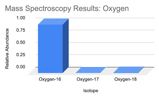
| Isotope | Relative Abundance |
| Oxygen-16 | 0.98757 |
| Oxygen-17 | 0.0021 |
| Oxygen-18 | 0.0104 |
Solution
\( \text { Average Atomic Mass } \left.=\sum \text { (relative abundance of isotope } n\right) \times(\text { mass of isotope } n) \)
Average atomic mass = (16)(0.98757) + (17)(0.0021) + (18)(0.0104)
Average atomic mass = 16.024 amu
The average atomic mass of this sample is 16.024 amu. Compared to the average atomic mass of oxygen on the periodic table of 15.9994 amu, it can be assumed that this particular sample contains a higher isotopic abundance of Oxygen-18 and Oxygen-17 than in nature.
Properties of Oxygen Based on Isotopic Mass
In nature, oxygen is commonly found in water molecules. These water molecules can be made with “heavy” oxygen (Oxygen-18) or “light” oxygen (Oxygen-16). Water molecules are held together through intermolecular forces called hydrogen bonds.
Water containing Oxygen-18 forms stronger hydrogen bonds than water containing Oxygen-16, so more energy is necessary to cause evaporation in water with Oxygen-18 than water with Oxygen-16.2 For this reason, water with Oxygen-16 evaporates more readily. Additionally, because of these stronger attractive forces, water molecules containing Oxygen-18 will condensate more readily than those with Oxygen-16. This is because in the gas form, the exothermic process of condensation releases more energy when water molecules with Oxygen-18 condense than when water molecules with Oxygen-16 condense.2-3
Therefore, in large bodies of water that contain both Oxygen-16 and Oxygen-18, water molecules with Oxygen-16 evaporate before those containing Oxygen-18 as temperature increases. Additionally, when temperature decreases, the water molecules with Oxygen-18 condense more readily.2
Putting these two factors together, it can be observed that: 1) Oxygen-16 is carried away from warmer areas as water vapor and 2) the concentration of Oxygen-18 in rainfall is high in warm areas, resulting in very little Oxygen-18 arriving in colder areas. Therefore, the trend in the image below is seen: warmer regions contain more Oxygen-18.2

Figure 2. Graph showing positive correlation between percent Oxygen-18 and Temperature. Source: NASA Earth Observatory.2
Oxygen Isotopes in Ice Cores and Ocean Water
Oxygen-18 can be the key in paleoclimate studies in observing how temperatures in certain regions have changed over time.2 The concentration of different oxygen isotopes in ice cores and ocean water can be linked to key findings due to the different properties of oxygen isotopes.
In terms of ice cores, ice in historically colder areas contains less concentration of Oxygen-18 relative to Oxygen-16.2 This is because Oxygen-18 evaporates more readily in warmer areas, and is precipitated in these warmer areas in the form of ice. In colder areas, however, this process happens more readily with Oxygen-16.
Isotope concentration in ocean water demonstrates the opposite trend: ocean water in colder areas contain a greater concentration of Oxygen-18 in comparison to Oxygen-16.4 Because Oxygen-18 evaporates less in colder areas, less Oxygen-18 is taken out of the ocean water, leaving a greater concentration in the ocean water. Additionally, Oxygen-18 condenses more in warmer areas, so when water vapor arrives in a colder area, most of the Oxygen-18 has already precipitated out. Therefore, precipitation in colder areas consists mostly of Oxygen-16, which then solidifies into the ice cores.2
Ice cores in colder areas contain less Oxygen-18 relative to Oxygen-16. Ocean water in colder areas contain more Oxygen-18 relative to Oxygen-16.
Link Between Oxygen Isotopes and Climate Change
These links between oxygen isotopic abundance and temperature can tell a story about the history of climate change across the world. In the field of paleoclimatology, researchers can use ice cores, which hold hundreds of years of data, in order to track these temperature changes over time.4 First, they can use mass spectroscopy to find the relative abundance of Oxygen-18 in comparison to Oxygen-16. With this data, the sample ratio of the relative concentration of these isotopes (Oxygen-18:Oxygen-16) can be calculated and then compared to the standard isotopic ratio of Standard Mean Ocean Water, which is 2005.20 ± 0.43 parts per million.5 Using the equation in the image below, the sample ratio of O18:O16 and the standard ratio of O18:O16 can be compared to find a sample-standard value for Oxygen-18 levels.
\[ δ^{18}O_{sample-standard} =1000\cfrac{\cfrac{^{18}O}{^{16}O}_{sample}-\cfrac{^{18}O}{^{16}O}_{standard}}{\cfrac{^{18}O}{^{16}O}_{standard}} =1000\cfrac{\cfrac{^{18}O}{^{16}O}_{sample}}{\cfrac{^{18}O}{^{16}O}_{standard}} -1\nonumber\]
Figure 3. Equation demonstrating how to calculate sample-standard value for Oxygen-18 levels. Source: ESS 312 Geochemistry.6
This analysis allows scientists to visualize trends in temperature over time as a result of climate change in one particular area and can be used to make predictions for temperature changes in the future.4 Because of the relationship between the isotopes and temperature previously detailed, higher concentrations of Oxygen-18 in ice cores are associated with higher regional temperatures during a period. The changes in concentration of Oxygen-18 in an ice core can be used to track temperature fluctuations throughout history.7
This analysis can also be done with ocean water isotope levels. Because areas with colder climates contain a lower concentration of Oxygen-18 in ice cores, there is relatively more Oxygen-18 in the ocean water in colder areas than there are in the ice cores. During periods of time when ice may be melting or the temperatures are rising, ice melts in colder areas, bringing Oxygen-16 into the ocean water and lowering the relative concentration of Oxygen-18 in the ocean water.7
Using the results of mass spectroscopy and the relationship between delta Oxygen-18 and temperature, estimate temperature during formation for Year X in Greenland.

| Oxygen-16 | Oxygen-18 | |
| Intensity | 5000000 | 9686 |

Figure 4. Graph showing positive correlation between average yearly temperature and delta Oxygen-18. Source: "How can Several Hundred Thousand Years of Temperature Data be Determined from Ice Core Samples?".8
Solution
First, calculate this sample of oxygen’s isotopic abundance. Remember that Oxygen-17 is not taken into consideration in paleoclimate studies due to its relatively low abundance.
Oxygen-16: (5000000)/(5000000 + 9686) = 0.9980665455
Oxygen-18: (9686)/(5000000 + 9686) = 0.0019334545
Ratio of the sample: (O-18/O-16) = (9686/5000000) = 0.0019372
Ratio of the standard VSMOW: 2005.20 ± .43 ppm, or the proportion 0.00200523
\[ δ^{18}O_{sample-standard} =1000\cfrac{\cfrac{^{18}O}{^{16}O}_{sample}-\cfrac{^{18}O}{^{16}O}_{standard}}{\cfrac{^{18}O}{^{16}O}_{standard}} =1000\cfrac{0.0019372-0.00200523}{0.00200523} =-33.92628277\nonumber\]
Using the graph provided, this delta Oxygen-18 value can be translated into an estimated temperature for Year X ice core formation of around -30.5℃. This calculation could then be compared to other delta Oxygen-18 values in history to determine temperature changes over time and make models for future predictions.
References
1. Khan Academy. Isotopes and mass spectrometry. https://www.khanacademy.org/science/...s-spectrometry (accessed 2022-10-30).
2. NASA. Paleoclimatology: The Oxygen Balance. https://earthobservatory.nasa.gov/fe..._OxygenBalance. (accessed 2022-27-10).
3. Wikipedia. Oxygen Isotope Ratio Cycle. https://en.m.wikipedia.org/wiki/Oxyg...pe_ratio_cycle (accessed 2022-10-30).
4. A Brief Explanation of Oxygen Isotopes in Paleoclimate Studies. https://pages.uoregon.edu/rdorsey/ge...-isotopes.html (accessed 2022-10-30).
5. Wikipedia. Vienna Standard Mean Ocean Water. https://en.wikipedia.org/wiki/Vienna...ture_standards. (accessed 2022-10-31).
6. ESS 312 Geochemistry. http://faculty.washington.edu/stn/es...re_notes.shtml (accessed 2022-11-02).
7. Climate Science Investigations South Florida - Temperature Over Time. Temperature over Time. http://www.ces.fau.edu/nasa/module-3...d/isotopes.php (accessed 2022-11-01).
8. Isotope Ratio Mass Spectrometry. How Can Several Hundred Thousand Years of Temperature Data Be Determined from Ice Core Samples?. https://applets.kcvs.ca/IsotopeRatio...ceCores-5.html. (accessed 2022-11-01).