2.1: Overview of Analytical Separations

In Chapter 7 we examined several methods for separating an analyte from potential interferents. For example, in a liquid–liquid extraction the analyte and interferent initially are present in a single liquid phase. We add a second, immiscible liquid phase and thoroughly mix them by shaking. During this process the analyte and interferents partition between the two phases to different extents, effecting their separation. After allowing the phases to separate, we draw off the phase enriched in analyte. Despite the power of liquid–liquid extractions, there are significant limitations.

Two Limitations of Liquid-Liquid Extractions

Suppose we have a sample that contains an analyte in a matrix that is incompatible with our analytical method. To determine the analyte’s concentration we first separate it from the matrix using a simple liquid–liquid extraction. If we have several analytes, we may need to complete a separate extraction for each analyte. For a complex mixture of analytes this quickly becomes a tedious process. This is one limitation to a liquid–liquid extraction.

A more significant limitation is that the extent of a separation depends on the distribution ratio of each species in the sample. If the analyte’s distribution ratio is similar to that of another species, then their separation becomes impossible. For example, let’s assume that an analyte, A, and an interferent, I, have distribution ratios of, respectively, 5 and 0.5. If we use a liquid–liquid extraction with equal volumes of sample and extractant, then it is easy to show that a single extraction removes approximately 83% of the analyte and 33% of the interferent. Although we can remove 99% of the analyte with three extractions, we also remove 70% of the interferent. In fact, there is no practical combination of number of extractions or volumes of sample and extractant that produce an acceptable separation.

From Chapter 7 we know that the distribution ratio, D, for a solute, S, is

\[D=\frac{[S]_{\mathrm{ext}}}{[S]_{\mathrm{samp}}} \nonumber\]

where [S]_ext is its equilibrium concentration in the extracting phase and [S]_samp is its equilibrium concentration in the sample. We can use the distribution ratio to calculate the fraction of S that remains in the sample, q_samp, after an extraction

\[q_{\text {samp}}=\frac{V_{\text {samp }}}{D V_{\text {ext }}+V_{\text {samp }}} \nonumber\]

where V_samp is the volume of sample and V_ext is the volume of the extracting phase. For example, if D = 10, V_samp = 20, and V_ext = 5, the fraction of S remaining in the sample after the extraction is

\[q_{\text { sanp }}=\frac{20}{10 \times 5+20}=0.29 \nonumber\]

or 29%. The remaining 71% of the analyte is in the extracting phase.

A Better Way to Separate Mixtures

The problem with a liquid–liquid extraction is that the separation occurs in one direction only: from the sample to the extracting phase. Let’s take a closer look at the liquid–liquid extraction of an analyte and an interferent with distribution ratios of, respectively, 5 and 0.5. Figure 12.1.1 shows that a single extraction using equal volumes of sample and extractant transfers 83% of the analyte and 33% of the interferent to the extracting phase. If the original concentrations of A and I are identical, then their concentration ratio in the extracting phase after one extraction is

\[\frac{[A]}{[I]}=\frac{0.83}{0.33}=2.5 \nonumber\]

A single extraction, therefore, enriches the analyte by a factor of \(2.5 \times\). After completing a second extraction (Figure 12.1.1 ) and combining the two extracting phases, the separation of the analyte and the interferent, surprisingly, is less efficient.

\[\frac{[A]}{[I]}=\frac{0.97}{0.55}=1.8 \nonumber\]

Figure 12.1.1 makes it clear why the second extraction results in a poorer overall separation: the second extraction actually favors the interferent!

Figure 12.1.1 . Progress of a traditional liquid–liquid extraction using two identical extractions of a single sample using fresh portions of the extractant. The numbers give the fraction of analyte and interferent in each phase assuming equal volumes of sample and extractant and distribution ratios of 5 and 0.5 for the analyte and the interferent, respectively. The opacity of the colors equals the fraction of analyte and interferent present.

We can improve the separation by first extracting the solutes from the sample into the extracting phase and then extracting them back into a fresh portion of solvent that matches the sample’s matrix (Figure 12.1.2 ). Because the analyte has the larger distribution ratio, more of it moves into the extractant during the first extraction and less of it moves back to the sample phase during the second extraction. In this case the concentration ratio in the extracting phase after two extractions is significantly greater.

\[\frac{[A]}{[I]}=\frac{0.69}{0.11}=6.3 \nonumber\]

Figure 12.1.2 . Progress of a liquid–liquid extraction in which we first extract the solutes into the extracting phase and then extract them back into an analyte-free portion of the sample’s phase. The numbers give the fraction of analyte and interferent in each phase assuming equal volumes of sample and extractant and distribution ratios of 5 and 0.5 for the analyte and the interferent, respectively. The opacity of the colors equals the fraction of analyte and interferent present.

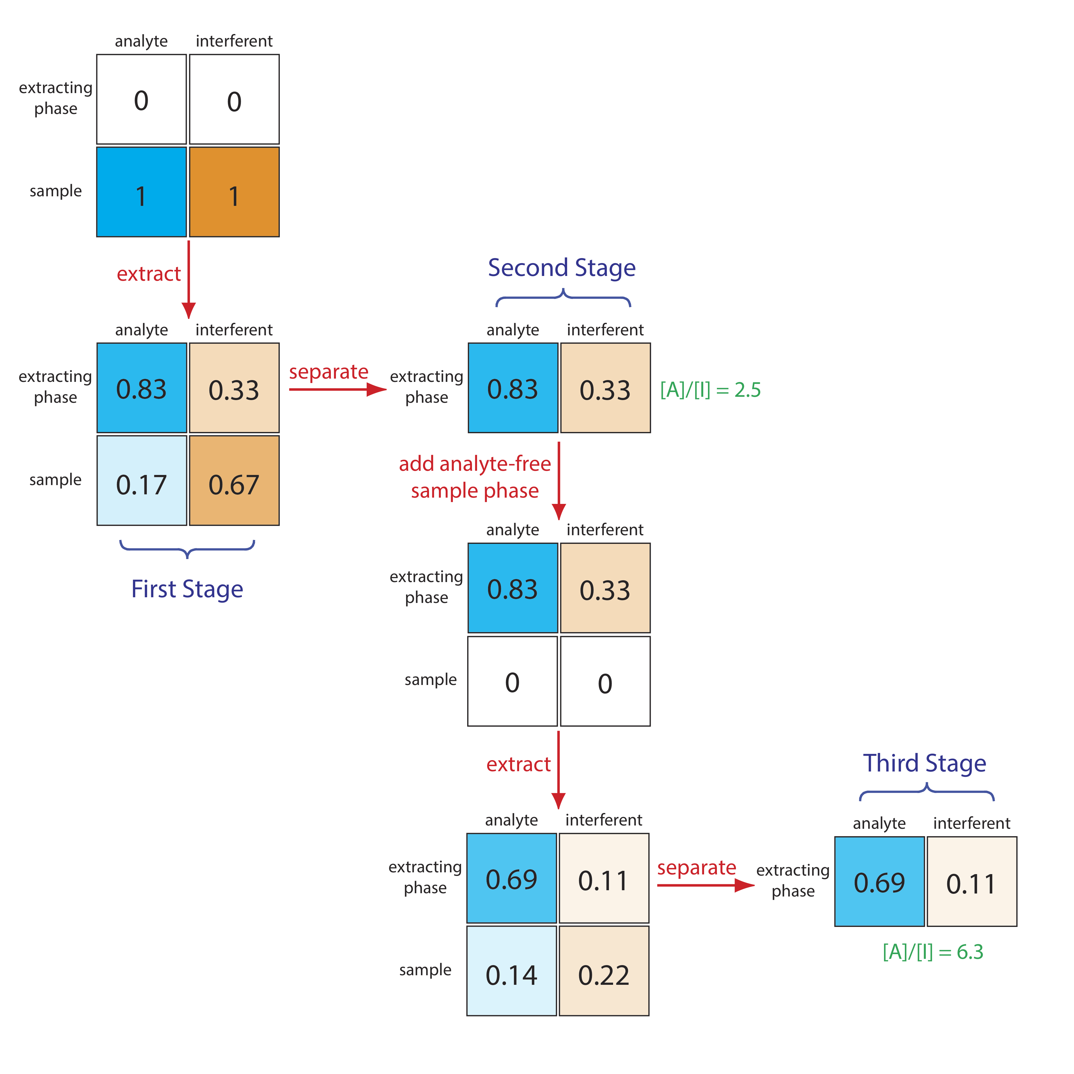
Not shown in Figure 12.2 is that we can add a fresh portion of the extracting phase to the sample that remains after the first extraction (the bottom row of the first stage in Figure 12.2, beginning the process anew. As we increase the number of extractions, the analyte and the interferent each spread out in space over a series of stages. Because the interferent’s distribution ratio is smaller than the analyte’s, the interferent lags behind the analyte. With a sufficient number of extractions—that is, a sufficient number of stages—a complete separation of the analyte and interferent is possible. This process of extracting the solutes back and forth between fresh portions of the two phases, which we call a countercurrent extraction, was developed by Craig in the 1940s [Craig, L. C. J. Biol. Chem. 1944, 155, 519–534]. The same phenomenon forms the basis of modern chromatography.

See Appendix 16 for a more detailed consideration of the mathematics behind a countercurrent extraction.

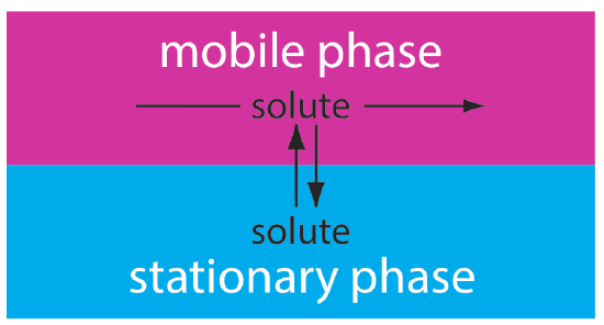
Chromatographic Separations

In chromatography we pass a sample-free phase, which we call the mobile phase, over a second sample-free stationary phase that remains fixed in space (Figure 12.1.3 ). We inject or place the sample into the mobile phase. As the sample moves with the mobile phase, its components partition between the mobile phase and the stationary phase. A component whose distribution ratio favors the stationary phase requires more time to pass through the system. Given sufficient time and sufficient stationary and mobile phase, we can separate solutes even if they have similar distribution ratios.

Figure 12.1.3 . In chromatography we pass a mobile phase over a stationary phase. When we inject a sample into the mobile phase, the sample’s components both move with the mobile phase and partition into the stationary phase. The solute that spends the most time in the stationary phase takes the longest time to move through the system.

There are many ways in which we can identify a chromatographic separation: by describing the physical state of the mobile phase and the stationary phase; by describing how we bring the stationary phase and the mobile phase into contact with each other; or by describing the chemical or physical interactions between the solute and the stationary phase. Let’s briefly consider how we might use each of these classifications.

We can trace the history of chromatography to the turn of the century when the Russian botanist Mikhail Tswett used a column packed with calcium carbonate and a mobile phase of petroleum ether to separate colored pigments from plant extracts. As the sample moved through the column, the plant’s pigments separated into individual colored bands. After effecting the separation, the calcium carbonate was removed from the column, sectioned, and the pigments recovered. Tswett named the technique chromatography, combining the Greek words for “color” and “to write.” There was little interest in Tswett’s technique until Martin and Synge’s pioneering development of a theory of chromatography (see Martin, A. J. P.; Synge, R. L. M. “A New Form of Chromatogram Employing Two Liquid Phases,” Biochem. J. 1941, 35, 1358–1366). Martin and Synge were awarded the 1952 Nobel Prize in Chemistry for this work.

Types of Mobile Phases and Stationary Phases

The mobile phase is a liquid or a gas, and the stationary phase is a solid or a liquid film coated on a solid substrate. We often name chromatographic techniques by listing the type of mobile phase followed by the type of stationary phase. In gas–liquid chromatography, for example, the mobile phase is a gas and the stationary phase is a liquid film coated on a solid substrate. If a technique’s name includes only one phase, as in gas chromatography, it is the mobile phase.

Contact Between the Mobile Phase and the Stationary Phase

There are two common methods for bringing the mobile phase and the stationary phase into contact. In column chromatography we pack the stationary phase into a narrow column and pass the mobile phase through the column using gravity or by applying pressure. The stationary phase is a solid particle or a thin liquid film coated on either a solid particulate packing material or on the column’s walls.

In planar chromatography the stationary phase is coated on a flat surface—typically, a glass, metal, or plastic plate. One end of the plate is placed in a reservoir that contains the mobile phase, which moves through the stationary phase by capillary action. In paper chromatography, for example, paper is the stationary phase.

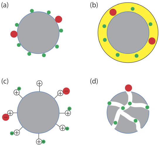
Interaction Between the Solute and the Stationary Phase

The interaction between the solute and the stationary phase provides a third method for describing a separation (Figure 12.1.4 ). In adsorption chromatography, solutes separate based on their ability to adsorb to a solid stationary phase. In partition chromatography, the stationary phase is a thin liquid film on a solid support. Separation occurs because there is a difference in the equilibrium partitioning of solutes between the stationary phase and the mobile phase. A stationary phase that consists of a solid support with covalently attached anionic (e.g., \(-\text{SO}_3^-\) ) or cationic (e.g., \(-\text{N(CH}_3)_3^+\)) functional groups is the basis for ion-exchange chromatography in which ionic solutes are attracted to the stationary phase by electrostatic forces. In size-exclusion chromatography the stationary phase is a porous particle or gel, with separation based on the size of the solutes. Larger solutes are unable to penetrate as deeply into the porous stationary phase and pass more quickly through the column.

Figure 12.1.4 . Four examples of interactions between a solute and the stationary phase: (a) adsorption on a solid surface, (b) partitioning into a liquid phase, (c) ion-exchange, and (d) size exclusion. For each example, the smaller, green solute is more strongly retained than the larger, red solute.

There are other interactions that can serve as the basis of a separation. In affinity chromatography the interaction between an antigen and an antibody, between an enzyme and a substrate, or between a receptor and a ligand forms the basis of a separation. See this chapter’s additional resources for some suggested readings.

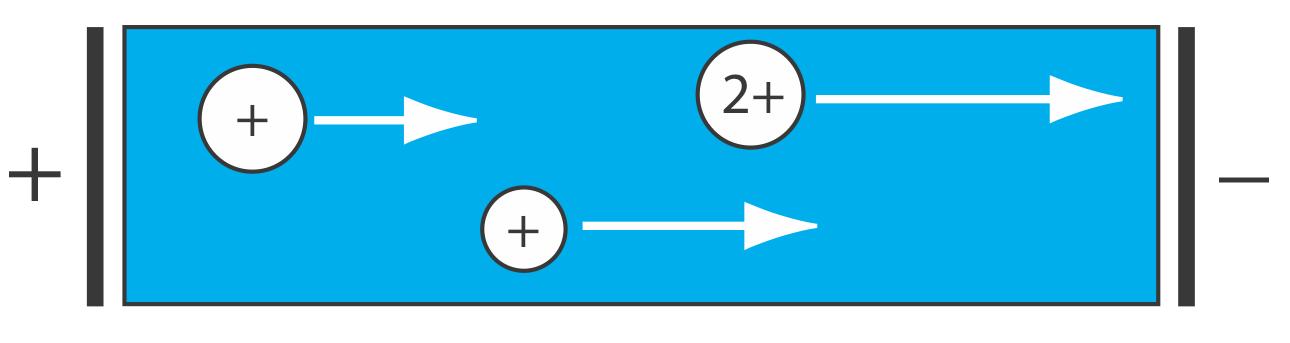
Electrophoretic Separations

In chromatography, a separation occurs because there is a difference in the equilibrium partitioning of solutes between the mobile phase and the stationary phase. Equilibrium partitioning, however, is not the only basis for effecting a separation. In an electrophoretic separation, for example, charged solutes migrate under the influence of an applied potential. A separation occurs because of differences in the charges and the sizes of the solutes (Figure 12.1.5 ).

Figure 12.1.5 . Movement of charged solutes under the influence of an applied potential. The lengths of the arrows indicate the relative speed of the solutes. In general, a larger solute moves more slowly than a smaller solute of equal charge, and a solute with a larger charge move more quickly than a solute with a smaller charge.