7.5: Quantum Mechanics and Atomic Orbitals

Learning Objectives

• To apply the results of quantum mechanics to chemistry.

The paradox described by Heisenberg’s uncertainty principle and the wavelike nature of subatomic particles such as the electron made it impossible to use the equations of classical physics to describe the motion of electrons in atoms. Scientists needed a new approach that took the wave behavior of the electron into account. In 1926, an Austrian physicist, Erwin Schrödinger (1887–1961; Nobel Prize in Physics, 1933), developed wave mechanics, a mathematical technique that describes the relationship between the motion of a particle that exhibits wavelike properties (such as an electron) and its allowed energies.

Erwin Schrödinger (1887–1961)

Schrödinger’s unconventional approach to atomic theory was typical of his unconventional approach to life. He was notorious for his intense dislike of memorizing data and learning from books. When Hitler came to power in Germany, Schrödinger escaped to Italy. He then worked at Princeton University in the United States but eventually moved to the Institute for Advanced Studies in Dublin, Ireland, where he remained until his retirement in 1955.

Although quantum mechanics uses sophisticated mathematics, you do not need to understand the mathematical details to follow our discussion of its general conclusions. We focus on the properties of the wave functions that are the solutions of Schrödinger’s equations.

Wave Functions

A wave function (Ψ) is a mathematical function that relates the location of an electron at a given point in space (identified by three spatial coordinates) to the amplitude of its wave, which corresponds to its energy. Thus each wave function is associated with a particular energy E. The properties of wave functions derived from quantum mechanics are summarized here:

• A wave function uses three variables to describe the position of an electron. A fourth variable is usually required to fully describe the location of objects in motion. Three specify the position in space (as with the Cartesian coordinates x, y, and z -or- Spherical coordinates (r, θ, φ) ), and one specifies the time at which the object is at the specified location. For example, if you were the captain of a ship trying to intercept an enemy submarine, you would need to know its latitude, longitude, and depth, as well as the time at which it was going to be at this position (Figure 6.5.1).

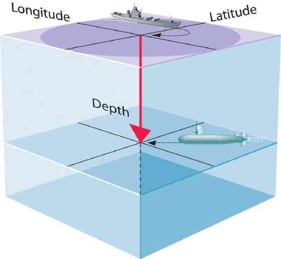
Figure \(\PageIndex{1}\): The Four Variables (Latitude, Longitude, Depth, and Time) required to precisely locate an object

For electrons, we will be using standing waves, which do not vary with time, to describe the position of an electron. Spherical coordinates (r, \(\theta\) and \(\phi\)) are commonly used when describing the position of an electron within an atom. We will often focus only on the radial component of the wave function! Note that the value of the r-coordinate tells us the distance of the electron from the nucleus (at r=0).

Figure \(\PageIndex{2}\): Spherical coordinates (r, θ, φ) as commonly used to locate an electron within an atom: radial distance r, polar angle θ (theta), and azimuthal angle φ (phi). (The symbol ρ (rho) is often used instead of r.)

• The magnitude of the wave function at a particular point in space is proportional to the amplitude of the wave at that point. Many wave functions are complex functions, which is a mathematical term indicating that they contain \(\sqrt{-1}\), represented as \(i\). Hence the amplitude of the wave has no real physical significance. In contrast, the sign of the wave function (either positive or negative) corresponds to the phase of the wave, which will be important in our discussion of chemical bonding. The sign of the wave function should not be confused with a positive or negative electrical charge.
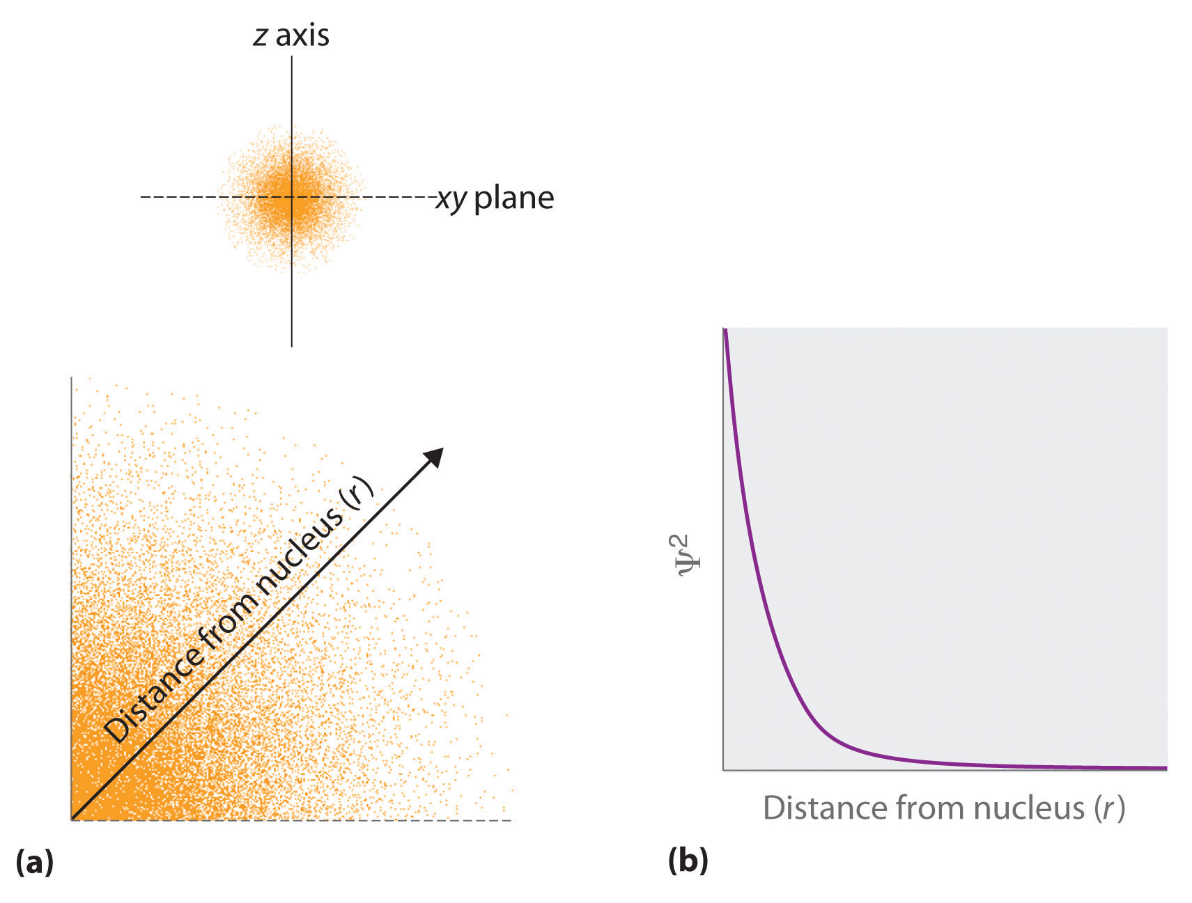
• The square of the wave function at a given point is proportional to the probability of finding an electron at that point, which leads to a distribution of probabilities in space. The square of the wave function (\(\Psi^2\)) is always a real quantity [recall that that \(\sqrt{-1}^2=-1\)] and is proportional to the probability of finding an electron at a given point. More accurately, the probability is given by the product of the wave function Ψ and its complex conjugate Ψ*, in which all terms that contain i are replaced by \(−i\). We use probabilities because, according to Heisenberg’s uncertainty principle, we cannot precisely specify the position of an electron. The probability of finding an electron at any point in space depends on several factors, including the distance from the nucleus and, in many cases, the atomic equivalent of latitude and longitude. As one way of graphically representing the probability distribution, the probability of finding an electron is indicated by the density of colored dots, as shown for the ground state of the hydrogen atom in Figure \(\PageIndex{2}\).
• Describing the electron distribution as a standing wave leads to sets of quantum numbers that are characteristic of each wave function. From the patterns of one- and two-dimensional standing waves shown previously, you might expect (correctly) that the patterns of three-dimensional standing waves would be complex. Fortunately, however, in the 18th century, a French mathematician, Adrien Legendre (1752–1783), developed a set of equations to describe the motion of tidal waves on the surface of a flooded planet. Schrödinger incorporated Legendre’s equations into his wave functions. The requirement that the waves must be in phase with one another to avoid cancelation and produce a standing wave results in a limited number of solutions (wave functions), each of which is specified by a set of numbers called quantum numbers.
• Each wave function is associated with a particular energy. As in Bohr’s model, the energy of an electron in an atom is quantized; it can have only certain allowed values. The major difference between Bohr’s model and Schrödinger’s approach is that Bohr had to impose the idea of quantization arbitrarily, whereas in Schrödinger’s approach, quantization is a natural consequence of describing an electron as a standing wave.

Figure \(\PageIndex{3}\): Probability of Finding the Electron in the Ground State of the Hydrogen Atom at Different Points in Space. (a) The density of the dots shows electron probability. (b) In this plot of Ψ² versus r for the ground state of the hydrogen atom, the electron probability density is greatest at r = 0 (the nucleus) and falls off with increasing r. Because the line never actually reaches the horizontal axis, the probability of finding the electron at very large values of r is very small but not zero.

Atomic Orbitals

You’ve probably seen the term “orbital” in previous chemistry classes. An orbital is a distribution for an electron. In other words, “an orbital” means “a map of where the electron tends to spend its time.” This map is provided by the wave function (Ψ), so “orbital” and “wave function” mean the same thing (more or less).

Visualizing an orbital can be tricky, because electrons can be just about anywhere. The electron in a hydrogen atom could be one foot away from the nucleus. However, this is extremely unlikely; the probability of the electron being that far away is around 10^{-2,502,324,325}. Electrons spend the vast majority of their time close to the nucleus. To depict an orbital, then, we can draw a picture of the region in which the electron spends 90% of its time; this is called the 90% contour.

We can only calculate wave functions for atoms with one electron, so we can only draw pictures of orbitals for one-electron atoms. When we do this for hydrogen, we notice a few things right away….

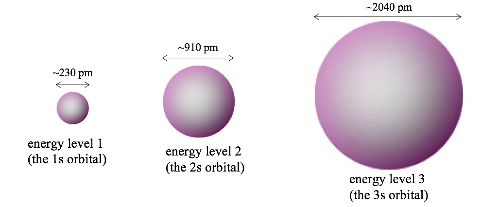
1) Orbitals that have different energies are always different sizes. For example, here are the 90% contours of the simplest-looking orbitals for energy levels 1, 2 and 3 in a hydrogen atom, along with the diameters of the 90% contours.

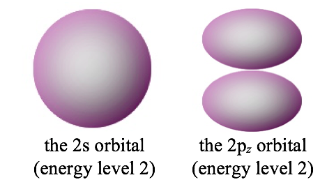
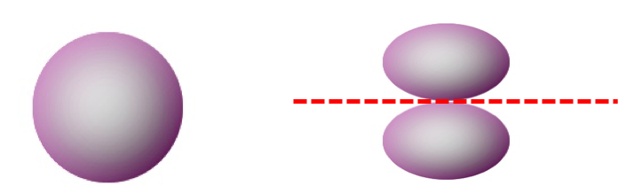
2) Some orbitals have the same energy, but are different shapes. For example, here are the 90% contours of two orbitals that have the same energy. Note that although their shapes are different, they are roughly the same size, because they have the same energy.

3) Most orbitals have at least one nodal surface. A nodal surface is a plane or a sphere on which the electron can never be found; the probability of the electron appearing on the nodal surface is zero. Nodal surfaces are directly connected with the energy of an orbital. The higher the energy of the orbital, the larger the number of nodal surfaces.

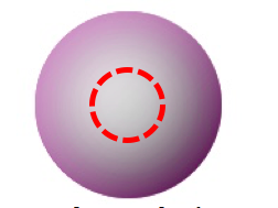
A spherical nodal surface is called a radial node, because you can describe it completely by telling what its radius is. When an orbital has a radial node, the electron can be inside the sphere, or outside the sphere, but never on the sphere. For example, the 2s orbital has a radial node, which is shown as a red dashed circle in the picture below. The electron spends about 5% of its time inside the red circle (actually a sphere) and 95% of its time outside the circle.

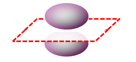
A planar nodal surface is called an angular node, because you can describe it by telling what angle it makes with one of the Cartesian axes. When an orbital has an angular node, the electron can be on either side of the plane, but never on it. For example, the 2p_z orbital has an angular node (a horizontal plane), as shown below. The plane extends infinitely far in all directions.

Orbitals can have more than one nodal surface. For example, the 3p_z orbital has two nodal surfaces: a radial node (a sphere) and an angular node (a plane).

Quantum Numbers

Schrödinger’s approach uses three quantum numbers (n, l, and m_l) to specify any wavefunction. You can think of them as a sort of shorthand notation for the wavefunction. The quantum numbers provide information about the spatial distribution of an electron. Although n can be any positive integer, only certain values of l and m_l are allowed for a given value of n.

The Principal Quantum Number

The principal quantum number (n) gives us a great deal of information about an orbital. It tells us…

• …the energy of the orbital
• …the relative size of the orbital (larger n = larger orbital)
• …the number of nodal surfaces that the orbital has (it’s always n – 1)

The name of any orbital always starts with the value of n. For a 1s orbital, n = 1, and for a 2p orbital, n = 2. The principal quantum number also tells us how many different orbitals (wave functions) have a particular energy. For any energy level, the total number of orbitals is n². For example, there are four different orbitals that have n = 2 (because 2² = 4) and nine different orbitals that have n = 3 (because 3² = 9).

There is no limit on the size of n; it can be any number from 1 to infinity. As n gets larger, the energy of the orbital gets larger (closer to zero) and the electron gets farther from the nucleus on average. When the energy reaches zero, the electron is completely removed from the atom.

\[n = 1, 2, 3, 4,… \label{7.5.1}\]

All wave functions that have the same value of n are said to constitute a principal shell because those electrons have similar average distances from the nucleus and energies. As you will see, the principal quantum number n corresponds to the n used by Bohr to describe electron orbits and by Rydberg to describe atomic energy levels.

The Azimuthal Quantum Number

The second quantum number is often called the azimuthal quantum number (l). The azimuthal quantum number tells us the general shape of an orbital. Specifically, it tells us the number of angular nodes that the orbital has. The angular nodes create the shape of an orbital. For instance, look at the difference between a 2s orbital (no angular nodes) and a 2p orbital (one angular node). Both orbitals have one nodal surface, but the 2s orbital has a radial node (a sphere), which is hidden inside the 90% contour, whereas the 2p orbital has an angular node, which chops the orbital into two pieces.

The value of l is always part of the orbital’s name, but it is “coded” in the following fashion:

If l = 0, we have an s orbital (1s, 2s, 3s, 4s, 5s…)

If l = 1, we have a p orbital (2p, 3p, 4p, 5p…)

If l = 2, we have a d orbital (3d, 4d, 5d…)

If l = 3, we have an f orbital (4f, 5f…)

The value of l also tells us how many orbitals of that type there are. If we specify both n and l, the total number of orbitals is 2l + 1. For example, there are five different 3d orbitals, because l = 2 for any kind of d orbital, and (2 × 2) + 1 = 5. The value of n doesn’t matter; there are also five different 4d orbitals, five different 5d orbitals, etc.

The value of l is limited by the value of n, because the number of angular nodes can’t be larger than the total number of nodes (which is n – 1). Therefore, l is always smaller than n. The allowed values of l depend on the value of n and can range from 0 to n − 1:

\[l = 0, 1, 2,…, n − 1 \label{7.5.2}\]

For example, if n = 1, l can be only 0; if n = 2, l can be 0 or 1; and so forth. For a given atom, all wave functions that have the same values of both n and l form a subshell. The regions of space occupied by electrons in the same subshell usually have the same shape, but they are oriented differently in space.

Example\(\PageIndex{1}\): Interpreting n and l

Here are some sample questions to illustrate the concepts we’ve looked at so far.

If n = 4, what are the possible values of l?

l can be 0, 1, 2 or 3.

What are the names of each of the orbitals that correspond to these combinations of n and l?

4s orbital (n = 4, l = 0), 4p orbital (n = 4, l = 1), 4d orbital (n = 4, l = 2), and 4f orbital (n = 4, l = 3).

How many nodes does each of these orbitals have? How many of them are angular and how many are radial?

All of these orbitals have 3 nodes, because the number of nodes equals n – 1, and n is 4 for all of these orbitals.

· The 4s orbital has l = 0, so it has no angular nodes. We already know that it has three nodes, so it must have three radial nodes.

· The 4p orbital has l = 1, so it has one angular node. Therefore, it must have two radial nodes.

· The 4d orbital has l = 2, so it has two angular nodes. Therefore, it must have one radial node.

· The 4f orbital has l = 3, so it has three angular nodes. Therefore, it has no radial nodes.

What is the energy of each of these orbitals?

These are hydrogen orbitals, so we can use the Bohr formula to calculate their energy. We know that all of them have n = 4, and the atomic number Z is 1 for hydrogen, so we have:

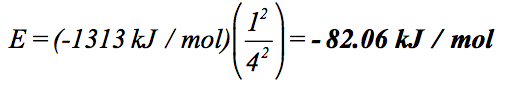
Note that all four of these orbitals have the same energy.

Rank these orbitals in order of size.

They are all approximately the same size, because they have the same value of n.

If an orbital has n = 7 and l = 2, what type of orbital is it?

It is a 7d orbital.

How many nodes does this orbital have? How many of them are radial nodes?

This orbital has six nodes, because the number of nodes equals n – 1, and 7 – 1 = 6. To find the number of radial nodes, we must find the number of angular nodes. The number of angular nodes always equals l, so this orbital has 2 angular nodes. Therefore, it has 6 – 2 = 4 radial nodes.

A hydrogen orbital has one angular node and four radial nodes. What kind of orbital is it?

This is a 6p orbital. It has one angular node, so l = 1, making it a p orbital. The total number of nodes is 1 + 4= 5, and this must equal n – 1, so n = 6 for this orbital.

A hydrogen orbital has five radial nodes, and its energy is -16.21 kJ/mol. What type of orbital is it?

We can calculate the value of n for this orbital, because we know its energy:

Solving for n gives n = 8.999965…, which we round to 9, since n must be a whole number. Next, we figure out the value of l. Since n = 9, this orbital has 8 nodes. We’re told that five of them are radial nodes, so the orbital has 8 – 5 = 3 angular nodes. Therefore, n = 9 and l = 3 for this orbital, making it a 9f orbital.

How many orbitals have n = 4?

There are 16 orbitals that have n = 4. The total number of orbitals that have a given value of n is n²; 4² = 16.

How many orbitals have n = 5 and l = 3?

There are 7 orbitals that have this combination of n and l. The number of orbitals that have a specific combination of n and l is 2l + 1; (2 × 3) + 1 = 7.

How many orbitals have n = 5 and l = 5?

No orbitals have this combination. l must always be smaller than n, because the total number of nodes is n – 1 and the number of angular nodes is l. Therefore, the largest possible value of l is n – 1.

How many 6s orbitals are there?

There is just one 6s orbital. For 6s orbitals, n = 6 and l = 0. The number of orbitals that has this combination of n and l is 2l + 1 = (2 × 0) + 1 = 1.

The Magnetic Quantum Number

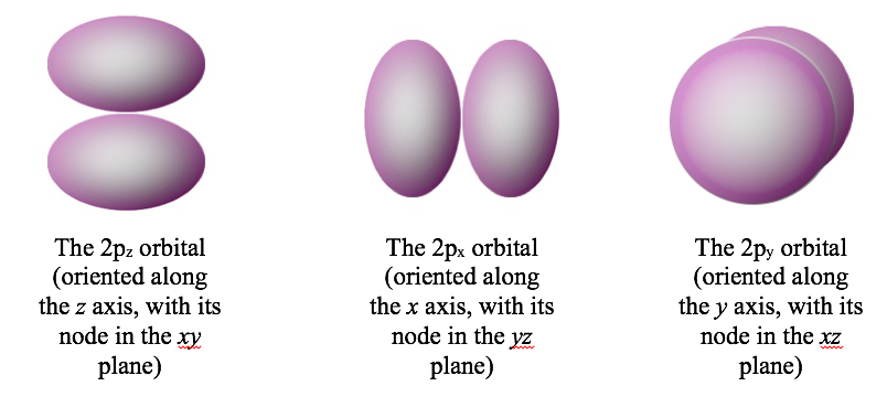
The third quantum number is the magnetic quantum number (\(m_l\)). The magnetic quantum number tells us the orientation of an orbital respect to an applied magnetic field.. More specifically, it tells us the orientation of the angular nodes. For example, a 2p orbital has one angular node, but that node can have three orientations: the xy plane, the xz plane, or the yz plane:

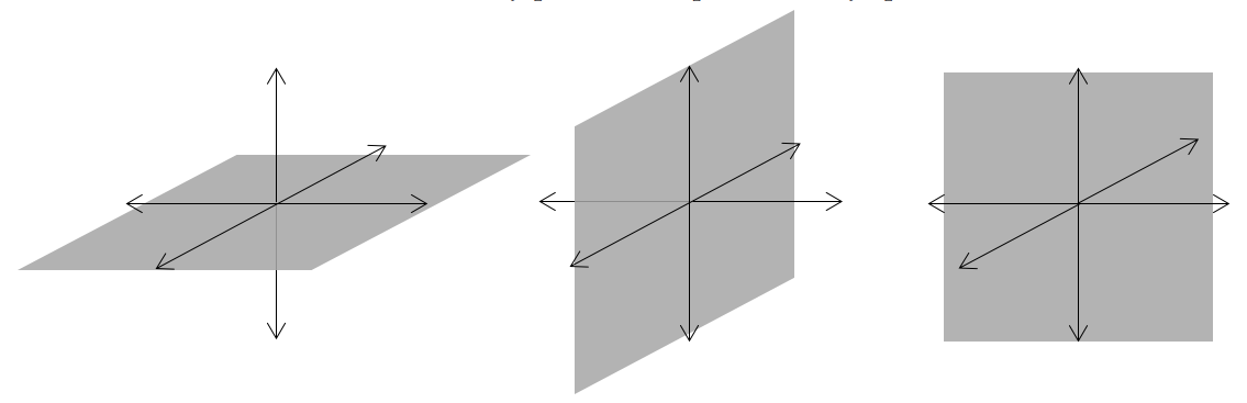
As a result, there are three different 2p orbitals, each oriented along one of the Cartesian axes.

The value of m_l determines the orientation of the orbital, essentially by determining how far the orbital is from the z axis. If the orbital is aligned along the z axis, m_l is zero. For the other orbitals, m_l is ±1; one of the orbitals has m_l = -1 and the other has m_l = 1. There is no fixed rule for this assignment though.

The possible values for m_l are controlled by the value of l. For a given value of l, m_l can be any integer from –l to +l. The allowed values of \(m_l\) therefore depend on the value of l: m_l can range from −l to l in integral steps:

\[m_l = −l, −l + 1,…, 0,…, l − 1, l \label{7.5.3}\]

For example, if l is 2 (i.e. if we are talking about d orbitals), m_l can be -2, -1, 0, 1, or 2. The number of options for m_l must match the total number of orbitals, which is 2l + 1; note that in this case, 2l + 1 = 5, and there are indeed five options for the value of m_l.

Each wave function with an allowed combination of n, l, and m_l values describes an atomic orbital, a particular spatial distribution for an electron. For a given set of quantum numbers, each principal shell has a fixed number of subshells, and each subshell has a fixed number of orbitals.

Example\(\PageIndex{2}\): n=4 Shell Structure

How many subshells and orbitals are contained within the principal shell with n = 4?

Given: value of n

Asked for: number of subshells and orbitals in the principal shell

Strategy:

1. Given n = 4, calculate the allowed values of l. From these allowed values, count the number of subshells.
2. For each allowed value of l, calculate the allowed values of m_l. The sum of the number of orbitals in each subshell is the number of orbitals in the principal shell.

Solution:

A We know that l can have all integral values from 0 to n − 1. If n = 4, then l can equal 0, 1, 2, or 3. Because the shell has four values of l, it has four subshells, each of which will contain a different number of orbitals, depending on the allowed values of m_l.

B For l = 0, m_l can be only 0, and thus the l = 0 subshell has only one orbital. For l = 1, m_l can be 0 or ±1; thus the l = 1 subshell has three orbitals. For l = 2, m_l can be 0, ±1, or ±2, so there are five orbitals in the l = 2 subshell. The last allowed value of l is l = 3, for which m_l can be 0, ±1, ±2, or ±3, resulting in seven orbitals in the l = 3 subshell. The total number of orbitals in the n = 4 principal shell is the sum of the number of orbitals in each subshell and is equal to n² = 16

Exercise \(\PageIndex{1}\): n=3 Shell Structure

How many subshells and orbitals are in the principal shell with n = 3?

Answer

three subshells; nine orbitals

We can summarize the relationships between the quantum numbers and the number of subshells and orbitals as follows (Table 7.5.1):

• Each principal shell has n subshells. For n = 1, only a single subshell is possible (1s); for n = 2, there are two subshells (2s and 2p); for n = 3, there are three subshells (3s, 3p, and 3d); and so forth. Every shell has an ns subshell, any shell with n ≥ 2 also has an np subshell, and any shell with n ≥ 3 also has an nd subshell. Because a 2d subshell would require both n = 2 and l = 2, which is not an allowed value of l for n = 2, a 2d subshell does not exist.
• Each subshell has 2l + 1 orbitals. This means that all ns subshells contain a single s orbital, all np subshells contain three p orbitals, all nd subshells contain five d orbitals, and all nf subshells contain seven f orbitals.

Table \(\PageIndex{1}\): Values of n, l, and ml through n = 4

n	l	Subshell Designation	\(m_l\)	Number of Orbitals in Subshell	Number of Orbitals in Shell
1	0	1s	0	1	1
2	0	2s	0	1	4
	1	2p	−1, 0, 1	3
3	0	3s	0	1	9
	1	3p	−1, 0, 1	3
	2	3d	−2, −1, 0, 1, 2	5
4	0	4s	0	1	16
	1	4p	−1, 0, 1	3
	2	4d	−2, −1, 0, 1, 2	5
	3	4f	−3, −2, −1, 0, 1, 2, 3	7

Example\(\PageIndex{2}\): The Three Quantum Numbers

Here are some sample questions that look at all three quantum numbers we’ve examined so far: n, l, and m_l.

What are the possible values of n, l, and m_l for a 13f orbital?

The name of the orbital tells us that n is 13 and l is 3. (Remember the “l code”: s, p, d, f corresponds to l = 0, 1, 2, 3.) Since l is 3, m_l can be any integer from -3 to +3, so the possible values of m_l are -3, -2, -1, 0, 1, 2 and 3.

An orbital has n = 4, l = 2, and m_l = -2. What kind of orbital is this?

This is a 4d orbital. The value of m_l tells us about the orientation of the orbital, but I don’t expect you to know which orbital corresponds to which value of m_l, so you can ignore m_l when you’re naming orbitals.

How many different orbitals have n = 6, l = 1, and m_l = 1?

Just one orbital has this combination. When you specify the values of all three quantum numbers, you have specified a single orbital.

How many different orbitals have n = 6 and m_l = 1?

This is a trickier question, because the question didn’t specify the value of l. We must consider all of the possible values of l that are compatible with n = 6 and m_l = 1…

n = 6, l = 0, m_l = 1 impossible, m_l can’t be larger than l

n = 6, l = 1, m_l = 1 okay – this is a 6p orbital

n = 6, l = 2, m_l = 1 okay – this is a 6d orbital

n = 6, l = 3, m_l = 1 okay – this is a 6f orbital

n = 6, l = 4, m_l = 1 okay – this is a 6g orbital (but you don't need to know that)

n = 6, l = 5, m_l = 1 okay – this is a 6h orbital (but you don’t need to know that)

n = 6, l = 6, m_l = 1 impossible, l must be smaller than n

l larger than 6 impossible, l must be smaller than n

Counting up the acceptable combinations, we see that there are five orbitals that have n = 6 and m_l = 1.

How many different orbitals have l = 3 and m_l = -2?

Infinite orbitals have this combination, because we didn’t specify the value of n. We know that n must be larger than l, but that just means that n can’t be 1, 2 or 3; it can still be any number from 4 to infinity. We could have a 4f orbital (n = 4, l = 3), a 5f orbital (n = 5, l = 3), a 6f orbital (n = 6, l = 3), etc. etc.

Summary

There is a relationship between the motions of electrons in atoms and molecules and their energies that is described by quantum mechanics. Because of wave–particle duality, scientists must deal with the probability of an electron being at a particular point in space. To do so required the development of quantum mechanics, which uses wave functions (Ψ) to describe the mathematical relationship between the motion of electrons in atoms and molecules and their energies. Wave functions have five important properties:

1. the wave function uses three spatial variables (Cartesian coordinates: x, y, and z -or- Spherical coordinates (r, θ, φ) ) to describe the position of an electron;
2. the magnitude of the wave function is proportional to the intensity of the wave;
3. the probability of finding an electron at a given point is proportional to the square of the wave function at that point, leading to a distribution of probabilities in space that is often portrayed as an electron density plot;
4. describing electron distributions as standing waves leads naturally to the existence of sets of quantum numbers characteristic of each wave function; and
5. each spatial distribution of the electron described by a wave function with a given set of quantum numbers has a particular energy.

Quantum numbers provide important information about the energy and spatial distribution of an electron. The principal quantum number n can be any positive integer; as n increases for an atom, the average distance of the electron from the nucleus also increases. All wave functions with the same value of n constitute a principal shell in which the electrons have similar average distances from the nucleus. The azimuthal quantum number l can have integral values between 0 and n − 1; it describes the shape of the electron distribution. Wave functions that have the same values of both n and l constitute a subshell, corresponding to electron distributions that usually differ in orientation rather than in shape or average distance from the nucleus. The magnetic quantum number m_l can have 2l + 1 integral values, ranging from −l to +l, and describes the orientation of the electron distribution. Each wave function with a given set of values of n, l, and m_l describes a particular spatial distribution of an electron in an atom, an atomic orbital.