1.6.2: The Kinetic-Molecular Theory
- Page ID
- 210613
\( \newcommand{\vecs}[1]{\overset { \scriptstyle \rightharpoonup} {\mathbf{#1}} } \)
\( \newcommand{\vecd}[1]{\overset{-\!-\!\rightharpoonup}{\vphantom{a}\smash {#1}}} \)
\( \newcommand{\id}{\mathrm{id}}\) \( \newcommand{\Span}{\mathrm{span}}\)
( \newcommand{\kernel}{\mathrm{null}\,}\) \( \newcommand{\range}{\mathrm{range}\,}\)
\( \newcommand{\RealPart}{\mathrm{Re}}\) \( \newcommand{\ImaginaryPart}{\mathrm{Im}}\)
\( \newcommand{\Argument}{\mathrm{Arg}}\) \( \newcommand{\norm}[1]{\| #1 \|}\)
\( \newcommand{\inner}[2]{\langle #1, #2 \rangle}\)
\( \newcommand{\Span}{\mathrm{span}}\)
\( \newcommand{\id}{\mathrm{id}}\)
\( \newcommand{\Span}{\mathrm{span}}\)
\( \newcommand{\kernel}{\mathrm{null}\,}\)
\( \newcommand{\range}{\mathrm{range}\,}\)
\( \newcommand{\RealPart}{\mathrm{Re}}\)
\( \newcommand{\ImaginaryPart}{\mathrm{Im}}\)
\( \newcommand{\Argument}{\mathrm{Arg}}\)
\( \newcommand{\norm}[1]{\| #1 \|}\)
\( \newcommand{\inner}[2]{\langle #1, #2 \rangle}\)
\( \newcommand{\Span}{\mathrm{span}}\) \( \newcommand{\AA}{\unicode[.8,0]{x212B}}\)
\( \newcommand{\vectorA}[1]{\vec{#1}} % arrow\)
\( \newcommand{\vectorAt}[1]{\vec{\text{#1}}} % arrow\)
\( \newcommand{\vectorB}[1]{\overset { \scriptstyle \rightharpoonup} {\mathbf{#1}} } \)
\( \newcommand{\vectorC}[1]{\textbf{#1}} \)
\( \newcommand{\vectorD}[1]{\overrightarrow{#1}} \)
\( \newcommand{\vectorDt}[1]{\overrightarrow{\text{#1}}} \)
\( \newcommand{\vectE}[1]{\overset{-\!-\!\rightharpoonup}{\vphantom{a}\smash{\mathbf {#1}}}} \)
\( \newcommand{\vecs}[1]{\overset { \scriptstyle \rightharpoonup} {\mathbf{#1}} } \)
\( \newcommand{\vecd}[1]{\overset{-\!-\!\rightharpoonup}{\vphantom{a}\smash {#1}}} \)
\(\newcommand{\avec}{\mathbf a}\) \(\newcommand{\bvec}{\mathbf b}\) \(\newcommand{\cvec}{\mathbf c}\) \(\newcommand{\dvec}{\mathbf d}\) \(\newcommand{\dtil}{\widetilde{\mathbf d}}\) \(\newcommand{\evec}{\mathbf e}\) \(\newcommand{\fvec}{\mathbf f}\) \(\newcommand{\nvec}{\mathbf n}\) \(\newcommand{\pvec}{\mathbf p}\) \(\newcommand{\qvec}{\mathbf q}\) \(\newcommand{\svec}{\mathbf s}\) \(\newcommand{\tvec}{\mathbf t}\) \(\newcommand{\uvec}{\mathbf u}\) \(\newcommand{\vvec}{\mathbf v}\) \(\newcommand{\wvec}{\mathbf w}\) \(\newcommand{\xvec}{\mathbf x}\) \(\newcommand{\yvec}{\mathbf y}\) \(\newcommand{\zvec}{\mathbf z}\) \(\newcommand{\rvec}{\mathbf r}\) \(\newcommand{\mvec}{\mathbf m}\) \(\newcommand{\zerovec}{\mathbf 0}\) \(\newcommand{\onevec}{\mathbf 1}\) \(\newcommand{\real}{\mathbb R}\) \(\newcommand{\twovec}[2]{\left[\begin{array}{r}#1 \\ #2 \end{array}\right]}\) \(\newcommand{\ctwovec}[2]{\left[\begin{array}{c}#1 \\ #2 \end{array}\right]}\) \(\newcommand{\threevec}[3]{\left[\begin{array}{r}#1 \\ #2 \\ #3 \end{array}\right]}\) \(\newcommand{\cthreevec}[3]{\left[\begin{array}{c}#1 \\ #2 \\ #3 \end{array}\right]}\) \(\newcommand{\fourvec}[4]{\left[\begin{array}{r}#1 \\ #2 \\ #3 \\ #4 \end{array}\right]}\) \(\newcommand{\cfourvec}[4]{\left[\begin{array}{c}#1 \\ #2 \\ #3 \\ #4 \end{array}\right]}\) \(\newcommand{\fivevec}[5]{\left[\begin{array}{r}#1 \\ #2 \\ #3 \\ #4 \\ #5 \\ \end{array}\right]}\) \(\newcommand{\cfivevec}[5]{\left[\begin{array}{c}#1 \\ #2 \\ #3 \\ #4 \\ #5 \\ \end{array}\right]}\) \(\newcommand{\mattwo}[4]{\left[\begin{array}{rr}#1 \amp #2 \\ #3 \amp #4 \\ \end{array}\right]}\) \(\newcommand{\laspan}[1]{\text{Span}\{#1\}}\) \(\newcommand{\bcal}{\cal B}\) \(\newcommand{\ccal}{\cal C}\) \(\newcommand{\scal}{\cal S}\) \(\newcommand{\wcal}{\cal W}\) \(\newcommand{\ecal}{\cal E}\) \(\newcommand{\coords}[2]{\left\{#1\right\}_{#2}}\) \(\newcommand{\gray}[1]{\color{gray}{#1}}\) \(\newcommand{\lgray}[1]{\color{lightgray}{#1}}\) \(\newcommand{\rank}{\operatorname{rank}}\) \(\newcommand{\row}{\text{Row}}\) \(\newcommand{\col}{\text{Col}}\) \(\renewcommand{\row}{\text{Row}}\) \(\newcommand{\nul}{\text{Nul}}\) \(\newcommand{\var}{\text{Var}}\) \(\newcommand{\corr}{\text{corr}}\) \(\newcommand{\len}[1]{\left|#1\right|}\) \(\newcommand{\bbar}{\overline{\bvec}}\) \(\newcommand{\bhat}{\widehat{\bvec}}\) \(\newcommand{\bperp}{\bvec^\perp}\) \(\newcommand{\xhat}{\widehat{\xvec}}\) \(\newcommand{\vhat}{\widehat{\vvec}}\) \(\newcommand{\uhat}{\widehat{\uvec}}\) \(\newcommand{\what}{\widehat{\wvec}}\) \(\newcommand{\Sighat}{\widehat{\Sigma}}\) \(\newcommand{\lt}{<}\) \(\newcommand{\gt}{>}\) \(\newcommand{\amp}{&}\) \(\definecolor{fillinmathshade}{gray}{0.9}\)The gas laws that we have seen to this point, as well as the ideal gas equation, are empirical, that is, they have been derived from experimental observations. The mathematical forms of these laws closely describe the macroscopic behavior of most gases at pressures less than about 1 or 2 atm. Although the gas laws describe relationships that have been verified by many experiments, they do not tell us why gases follow these relationships.
The kinetic molecular theory (KMT) is a simple microscopic model that effectively explains the gas laws described in previous modules of this chapter. This theory is based on the following five postulates described here. (Note: The term “molecule” will be used to refer to the individual chemical species that compose the gas, although some gases are composed of atomic species, for example, the noble gases.)
- The molecules composing the gas are negligibly small compared to the distances between them.
- Gas molecules exert no attractive or repulsive forces on each other or the container walls; therefore, their collisions are elastic (do not involve a loss of energy).
- The average kinetic energy of the gas molecules is proportional to the kelvin temperature of the gas.
The test of the KMT and its postulates is its ability to explain and describe the behavior of a gas. The various gas laws can be derived from the assumptions of the KMT, which have led chemists to believe that the assumptions of the theory accurately represent the properties of gas molecules. We will first look at the individual gas laws (Boyle’s, Charles’s, Amontons’s, Avogadro’s, and Dalton’s laws) conceptually to see how the KMT explains them. Then, we will more carefully consider the relationships between molecular masses, speeds, and kinetic energies with temperature, and explain Graham’s law.
The Kinetic-Molecular Theory Explains the Behavior of Gases
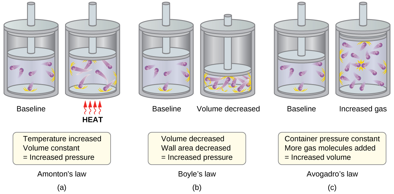
Recalling that gas pressure is exerted by rapidly moving gas molecules and depends directly on the number of molecules hitting a unit area of the wall per unit of time, we see that the KMT conceptually explains the behavior of a gas as follows:
- Charles’s law. If the temperature of a gas is increased, a constant pressure may be maintained only if the volume occupied by the gas increases. This will result in greater average distances traveled by the molecules to reach the container walls, as well as increased wall surface area. These conditions will decrease both the frequency of molecule-wall collisions and the number of collisions per unit area, the combined effects of which balance the effect of increased collision forces due to the greater kinetic energy at the higher temperature.
- Avogadro’s law. At constant pressure and temperature, the frequency and force of molecule-wall collisions are constant. Under such conditions, increasing the number of gaseous molecules will require a proportional increase in the container volume in order to yield a decrease in the number of collisions per unit area to compensate for the increased frequency of collisions (Figure \(\PageIndex{1c}\)).
- Dalton’s Law. Because of the large distances between them, the molecules of one gas in a mixture bombard the container walls with the same frequency whether other gases are present or not, and the total pressure of a gas mixture equals the sum of the (partial) pressures of the individual gases.

Summary
The kinetic molecular theory is a simple but very effective model that effectively explains ideal gas behavior. The theory assumes that gases consist of widely separated molecules of negligible volume that are in constant motion, colliding elastically with one another and the walls of their container with average velocities determined by their absolute temperatures. The individual molecules of a gas exhibit a range of velocities, the distribution of these velocities being dependent on the temperature of the gas and the mass of its molecules.
Glossary
- kinetic molecular theory
- theory based on simple principles and assumptions that effectively explains ideal gas behavior
Contributors and Attributions
Paul Flowers (University of North Carolina - Pembroke), Klaus Theopold (University of Delaware) and Richard Langley (Stephen F. Austin State University) with contributing authors. Textbook content produced by OpenStax College is licensed under a Creative Commons Attribution License 4.0 license. Download for free at http://cnx.org/contents/85abf193-2bd...a7ac8df6@9.110).


