
10.4: Colligative Properties
- Page ID
- 162497

\( \newcommand{\vecs}[1]{\overset { \scriptstyle \rightharpoonup} {\mathbf{#1}} } \)
\( \newcommand{\vecd}[1]{\overset{-\!-\!\rightharpoonup}{\vphantom{a}\smash {#1}}} \)
\( \newcommand{\id}{\mathrm{id}}\) \( \newcommand{\Span}{\mathrm{span}}\)
( \newcommand{\kernel}{\mathrm{null}\,}\) \( \newcommand{\range}{\mathrm{range}\,}\)
\( \newcommand{\RealPart}{\mathrm{Re}}\) \( \newcommand{\ImaginaryPart}{\mathrm{Im}}\)
\( \newcommand{\Argument}{\mathrm{Arg}}\) \( \newcommand{\norm}[1]{\| #1 \|}\)
\( \newcommand{\inner}[2]{\langle #1, #2 \rangle}\)
\( \newcommand{\Span}{\mathrm{span}}\)
\( \newcommand{\id}{\mathrm{id}}\)
\( \newcommand{\Span}{\mathrm{span}}\)
\( \newcommand{\kernel}{\mathrm{null}\,}\)
\( \newcommand{\range}{\mathrm{range}\,}\)
\( \newcommand{\RealPart}{\mathrm{Re}}\)
\( \newcommand{\ImaginaryPart}{\mathrm{Im}}\)
\( \newcommand{\Argument}{\mathrm{Arg}}\)
\( \newcommand{\norm}[1]{\| #1 \|}\)
\( \newcommand{\inner}[2]{\langle #1, #2 \rangle}\)
\( \newcommand{\Span}{\mathrm{span}}\) \( \newcommand{\AA}{\unicode[.8,0]{x212B}}\)
\( \newcommand{\vectorA}[1]{\vec{#1}} % arrow\)
\( \newcommand{\vectorAt}[1]{\vec{\text{#1}}} % arrow\)
\( \newcommand{\vectorB}[1]{\overset { \scriptstyle \rightharpoonup} {\mathbf{#1}} } \)
\( \newcommand{\vectorC}[1]{\textbf{#1}} \)
\( \newcommand{\vectorD}[1]{\overrightarrow{#1}} \)
\( \newcommand{\vectorDt}[1]{\overrightarrow{\text{#1}}} \)
\( \newcommand{\vectE}[1]{\overset{-\!-\!\rightharpoonup}{\vphantom{a}\smash{\mathbf {#1}}}} \)
\( \newcommand{\vecs}[1]{\overset { \scriptstyle \rightharpoonup} {\mathbf{#1}} } \)
\( \newcommand{\vecd}[1]{\overset{-\!-\!\rightharpoonup}{\vphantom{a}\smash {#1}}} \)
\(\newcommand{\avec}{\mathbf a}\) \(\newcommand{\bvec}{\mathbf b}\) \(\newcommand{\cvec}{\mathbf c}\) \(\newcommand{\dvec}{\mathbf d}\) \(\newcommand{\dtil}{\widetilde{\mathbf d}}\) \(\newcommand{\evec}{\mathbf e}\) \(\newcommand{\fvec}{\mathbf f}\) \(\newcommand{\nvec}{\mathbf n}\) \(\newcommand{\pvec}{\mathbf p}\) \(\newcommand{\qvec}{\mathbf q}\) \(\newcommand{\svec}{\mathbf s}\) \(\newcommand{\tvec}{\mathbf t}\) \(\newcommand{\uvec}{\mathbf u}\) \(\newcommand{\vvec}{\mathbf v}\) \(\newcommand{\wvec}{\mathbf w}\) \(\newcommand{\xvec}{\mathbf x}\) \(\newcommand{\yvec}{\mathbf y}\) \(\newcommand{\zvec}{\mathbf z}\) \(\newcommand{\rvec}{\mathbf r}\) \(\newcommand{\mvec}{\mathbf m}\) \(\newcommand{\zerovec}{\mathbf 0}\) \(\newcommand{\onevec}{\mathbf 1}\) \(\newcommand{\real}{\mathbb R}\) \(\newcommand{\twovec}[2]{\left[\begin{array}{r}#1 \\ #2 \end{array}\right]}\) \(\newcommand{\ctwovec}[2]{\left[\begin{array}{c}#1 \\ #2 \end{array}\right]}\) \(\newcommand{\threevec}[3]{\left[\begin{array}{r}#1 \\ #2 \\ #3 \end{array}\right]}\) \(\newcommand{\cthreevec}[3]{\left[\begin{array}{c}#1 \\ #2 \\ #3 \end{array}\right]}\) \(\newcommand{\fourvec}[4]{\left[\begin{array}{r}#1 \\ #2 \\ #3 \\ #4 \end{array}\right]}\) \(\newcommand{\cfourvec}[4]{\left[\begin{array}{c}#1 \\ #2 \\ #3 \\ #4 \end{array}\right]}\) \(\newcommand{\fivevec}[5]{\left[\begin{array}{r}#1 \\ #2 \\ #3 \\ #4 \\ #5 \\ \end{array}\right]}\) \(\newcommand{\cfivevec}[5]{\left[\begin{array}{c}#1 \\ #2 \\ #3 \\ #4 \\ #5 \\ \end{array}\right]}\) \(\newcommand{\mattwo}[4]{\left[\begin{array}{rr}#1 \amp #2 \\ #3 \amp #4 \\ \end{array}\right]}\) \(\newcommand{\laspan}[1]{\text{Span}\{#1\}}\) \(\newcommand{\bcal}{\cal B}\) \(\newcommand{\ccal}{\cal C}\) \(\newcommand{\scal}{\cal S}\) \(\newcommand{\wcal}{\cal W}\) \(\newcommand{\ecal}{\cal E}\) \(\newcommand{\coords}[2]{\left\{#1\right\}_{#2}}\) \(\newcommand{\gray}[1]{\color{gray}{#1}}\) \(\newcommand{\lgray}[1]{\color{lightgray}{#1}}\) \(\newcommand{\rank}{\operatorname{rank}}\) \(\newcommand{\row}{\text{Row}}\) \(\newcommand{\col}{\text{Col}}\) \(\renewcommand{\row}{\text{Row}}\) \(\newcommand{\nul}{\text{Nul}}\) \(\newcommand{\var}{\text{Var}}\) \(\newcommand{\corr}{\text{corr}}\) \(\newcommand{\len}[1]{\left|#1\right|}\) \(\newcommand{\bbar}{\overline{\bvec}}\) \(\newcommand{\bhat}{\widehat{\bvec}}\) \(\newcommand{\bperp}{\bvec^\perp}\) \(\newcommand{\xhat}{\widehat{\xvec}}\) \(\newcommand{\vhat}{\widehat{\vvec}}\) \(\newcommand{\uhat}{\widehat{\uvec}}\) \(\newcommand{\what}{\widehat{\wvec}}\) \(\newcommand{\Sighat}{\widehat{\Sigma}}\) \(\newcommand{\lt}{<}\) \(\newcommand{\gt}{>}\) \(\newcommand{\amp}{&}\) \(\definecolor{fillinmathshade}{gray}{0.9}\)Learning Objectives
- Describe the effect of solute concentration on various solution properties (vapor pressure, boiling point, freezing point, and osmotic pressure)
- Describe the process of distillation and its practical applications
- Explain the process of osmosis and describe how it is applied industrially and in nature
The properties of a solution are different from those of either the pure solute(s) or solvent. Many solution properties are dependent upon the chemical identity of the solute. Compared to pure water, a solution of hydrogen chloride is more acidic, a solution of ammonia is more basic, a solution of sodium chloride is more dense, and a solution of sucrose is more viscous. There are a few solution properties, however, that depend only upon the total concentration of solute species, regardless of their identities. These colligative properties include vapor pressure lowering, boiling point elevation, freezing point depression, and osmotic pressure. This small set of properties is of central importance to many natural phenomena and technological applications, as will be described in this module.
Vapor Pressure Lowering
As described in the chapter on liquids and solids, the equilibrium vapor pressure of a liquid is the pressure exerted by its gaseous phase when vaporization and condensation are occurring at equal rates:
\[ \text{liquid} \rightleftharpoons \text{gas} \label{11.5.4}\]
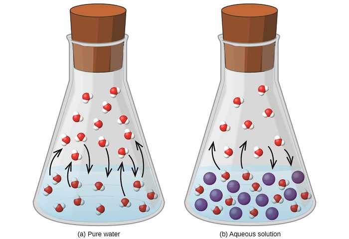
Dissolving a nonvolatile substance in a volatile liquid results in a lowering of the liquid’s vapor pressure. This phenomenon can be rationalized by considering the effect of added solute molecules on the liquid's vaporization and condensation processes. To vaporize, solvent molecules must be present at the surface of the solution. The presence of solute decreases the surface area available to solvent molecules and thereby reduces the rate of solvent vaporization. Since the rate of condensation is unaffected by the presence of solute, the net result is that the vaporization-condensation equilibrium is achieved with fewer solvent molecules in the vapor phase (i.e., at a lower vapor pressure) (Figure \(\PageIndex{1}\)). While this kinetic interpretation is useful, it does not account for several important aspects of the colligative nature of vapor pressure lowering. A more rigorous explanation involves the property of entropy, a topic of discussion in a later text chapter on thermodynamics. For purposes of understanding the lowering of a liquid's vapor pressure, it is adequate to note that the greater entropy of a solution in comparison to its separate solvent and solute serves to effectively stabilize the solvent molecules and hinder their vaporization. A lower vapor pressure results, and a correspondingly higher boiling point as described in the next section of this module.
Elevation of the Boiling Point of a Solvent
As described in the chapter on liquids and solids, the boiling point of a liquid is the temperature at which its vapor pressure is equal to ambient atmospheric pressure. Since the vapor pressure of a solution is lowered due to the presence of nonvolatile solutes, it stands to reason that the solution’s boiling point will subsequently be increased. Compared to pure solvent, a solution, therefore, will require a higher temperature to achieve any given vapor pressure, including one equivalent to that of the surrounding atmosphere. The extent to which the vapor pressure of a solvent is lowered and the boiling point is elevated depends on the total number of solute particles present in a given amount of solvent, not on the mass or size or chemical identities of the particles. A 1 m aqueous solution of sucrose (342 g/mol) and a 1 m aqueous solution of ethylene glycol (62 g/mol) will exhibit the same boiling point because each solution has one mole of solute particles (molecules) per kilogram of solvent.
Distillation of Solutions
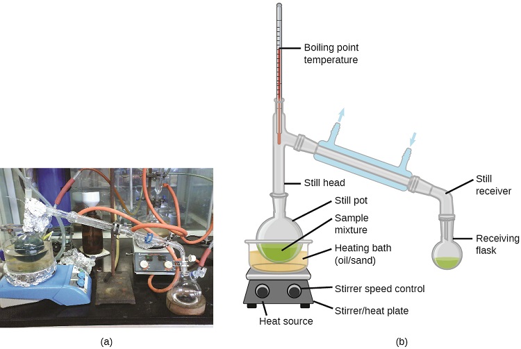
Distillation is a technique for separating the components of mixtures that is widely applied in both in the laboratory and in industrial settings. It is used to refine petroleum, to isolate fermentation products, and to purify water. This separation technique involves the controlled heating of a sample mixture to selectively vaporize, condense, and collect one or more components of interest. A typical apparatus for laboratory-scale distillations is shown in Figure \(\PageIndex{2}\).
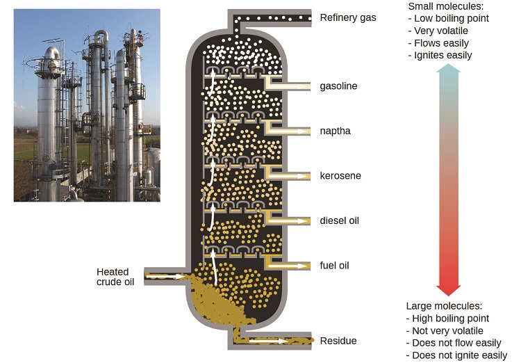
Oil refineries use large-scale fractional distillation to separate the components of crude oil. The crude oil is heated to high temperatures at the base of a tall fractionating column, vaporizing many of the components that rise within the column. As vaporized components reach adequately cool zones during their ascent, they condense and are collected. The collected liquids are simpler mixtures of hydrocarbons and other petroleum compounds that are of appropriate composition for various applications (e.g., diesel fuel, kerosene, gasoline), as depicted in Figure \(\PageIndex{3}\).
Depression of the Freezing Point of a Solvent
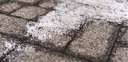
Solutions freeze at lower temperatures than pure liquids. This phenomenon is exploited in “de-icing” schemes that use salt (Figure \(\PageIndex{4}\)), calcium chloride, or urea to melt ice on roads and sidewalks, and in the use of ethylene glycol as an “antifreeze” in automobile radiators. Seawater freezes at a lower temperature than fresh water, and so the Arctic and Antarctic oceans remain unfrozen even at temperatures below 0 °C (as do the body fluids of fish and other cold-blooded sea animals that live in these oceans).
Colligative Properties and De-Icing
Sodium chloride and its group 2 analogs calcium and magnesium chloride are often used to de-ice roadways and sidewalks, due to the fact that a solution of any one of these salts will have a freezing point lower than 0 °C, the freezing point of pure water. The group 2 metal salts are frequently mixed with the cheaper and more readily available sodium chloride (“rock salt”) for use on roads, since they tend to be somewhat less corrosive than the NaCl, and they provide a larger depression of the freezing point, since they dissociate to yield three particles per formula unit, rather than two particles like the sodium chloride.
Because these ionic compounds tend to hasten the corrosion of metal, they would not be a wise choice to use in antifreeze for the radiator in your car or to de-ice a plane prior to takeoff. For these applications, covalent compounds, such as ethylene or propylene glycol, are often used. The glycols used in radiator fluid not only lower the freezing point of the liquid, but they elevate the boiling point, making the fluid useful in both winter and summer. Heated glycols are often sprayed onto the surface of airplanes prior to takeoff in inclement weather in the winter to remove ice that has already formed and prevent the formation of more ice, which would be particularly dangerous if formed on the control surfaces of the aircraft (Video \(\PageIndex{1}\)).
Video \(\PageIndex{1}\): Freezing point depression is exploited to remove ice from the control surfaces of aircraft.
Osmosis and Osmotic Pressure of Solutions
A number of natural and synthetic materials exhibit selective permeation, meaning that only molecules or ions of a certain size, shape, polarity, charge, and so forth, are capable of passing through (permeating) the material. Biological cell membranes provide elegant examples of selective permeation in nature, while dialysis tubing used to remove metabolic wastes from blood is a more simplistic technological example. Regardless of how they may be fabricated, these materials are generally referred to as semipermeable membranes.
Consider the apparatus illustrated in Figure \(\PageIndex{6}\), in which samples of pure solvent and a solution are separated by a membrane that only solvent molecules may permeate. Solvent molecules will diffuse across the membrane in both directions. Since the concentration of solvent is greater in the pure solvent than the solution, these molecules will diffuse from the solvent side of the membrane to the solution side at a faster rate than they will in the reverse direction. The result is a net transfer of solvent molecules from the pure solvent to the solution. Diffusion-driven transfer of solvent molecules through a semipermeable membrane is a process known as osmosis.
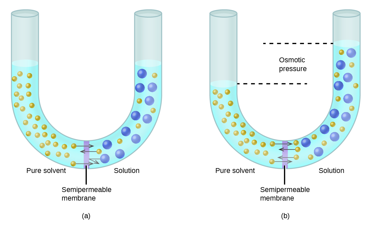
When osmosis is carried out in an apparatus like that shown in Figure \(\PageIndex{6}\), the volume of the solution increases as it becomes diluted by accumulation of solvent. This causes the level of the solution to rise, increasing its hydrostatic pressure (due to the weight of the column of solution in the tube) and resulting in a faster transfer of solvent molecules back to the pure solvent side. When the pressure reaches a value that yields a reverse solvent transfer rate equal to the osmosis rate, bulk transfer of solvent ceases. This pressure is called the osmotic pressure (\(\Pi\)) of the solution.
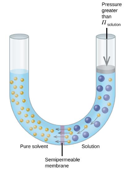
If a solution is placed in an apparatus like the one shown in Figure \(\PageIndex{7}\), applying pressure greater than the osmotic pressure of the solution reverses the osmosis and pushes solvent molecules from the solution into the pure solvent. This technique of reverse osmosis is used for large-scale desalination of seawater and on smaller scales to produce high-purity tap water for drinking.
Examples of osmosis are evident in many biological systems because cells are surrounded by semipermeable membranes. Carrots and celery that have become limp because they have lost water can be made crisp again by placing them in water. Water moves into the carrot or celery cells by osmosis. A cucumber placed in a concentrated salt solution loses water by osmosis and absorbs some salt to become a pickle. Osmosis can also affect animal cells. Solute concentrations are particularly important when solutions are injected into the body. Solutes in body cell fluids and blood serum give these solutions an osmotic pressure of approximately 7.7 atm. Solutions injected into the body must have the same osmotic pressure as blood serum; that is, they should be isotonic with blood serum. If a less concentrated solution, a hypotonic solution, is injected in sufficient quantity to dilute the blood serum, water from the diluted serum passes into the blood cells by osmosis, causing the cells to expand and rupture. This process is called hemolysis. When a more concentrated solution, a hypertonic solution, is injected, the cells lose water to the more concentrated solution, shrivel, and possibly die in a process called crenation (Figure 11.5.8).

Colligative Properties of Electrolytes
As noted previously in this module, the colligative properties of a solution depend only on the number, not on the kind, of solute species dissolved. For example, 1 mole of any nonelectrolyte dissolved in 1 kilogram of solvent produces the same lowering of the freezing point as does 1 mole of any other nonelectrolyte. However, 1 mole of sodium chloride (an electrolyte) forms 2 moles of ions when dissolved in solution. Each individual ion produces the same effect on the freezing point as a single molecule does.
Summary
Properties of a solution that depend only on the concentration of solute particles are called colligative properties. They include changes in the vapor pressure, boiling point, and freezing point of the solvent in the solution. The magnitudes of these properties depend only on the total concentration of solute particles in solution, not on the type of particles. The total concentration of solute particles in a solution also determines its osmotic pressure. This is the pressure that must be applied to the solution to prevent diffusion of molecules of pure solvent through a semipermeable membrane into the solution. Ionic compounds may not completely dissociate in solution due to activity effects, in which case observed colligative effects may be less than predicted.
Footnotes
- A nonelectrolyte shown for comparison.
Glossary
- boiling point elevation
- elevation of the boiling point of a liquid by addition of a solute
- colligative property
- property of a solution that depends only on the concentration of a solute species
- freezing point depression
- lowering of the freezing point of a liquid by addition of a solute
- hemolysis
- rupture of red blood cells due to the accumulation of excess water by osmosis
- hypertonic
- of greater osmotic pressure
- hypotonic
- of less osmotic pressure
- isotonic
- of equal osmotic pressure
- osmosis
- diffusion of solvent molecules through a semipermeable membrane
- osmotic pressure (Π)
- opposing pressure required to prevent bulk transfer of solvent molecules through a semipermeable membrane
- semipermeable membrane
- a membrane that selectively permits passage of certain ions or molecules
Contributors
Paul Flowers (University of North Carolina - Pembroke), Klaus Theopold (University of Delaware) and Richard Langley (Stephen F. Austin State University) with contributing authors. Textbook content produced by OpenStax College is licensed under a Creative Commons Attribution License 4.0 license. Download for free at http://cnx.org/contents/85abf193-2bd...a7ac8df6@9.110).