14.4: Using Excel and R for an Analysis of Variance
- Page ID
- 220785

\( \newcommand{\vecs}[1]{\overset { \scriptstyle \rightharpoonup} {\mathbf{#1}} } \)
\( \newcommand{\vecd}[1]{\overset{-\!-\!\rightharpoonup}{\vphantom{a}\smash {#1}}} \)
\( \newcommand{\id}{\mathrm{id}}\) \( \newcommand{\Span}{\mathrm{span}}\)
( \newcommand{\kernel}{\mathrm{null}\,}\) \( \newcommand{\range}{\mathrm{range}\,}\)
\( \newcommand{\RealPart}{\mathrm{Re}}\) \( \newcommand{\ImaginaryPart}{\mathrm{Im}}\)
\( \newcommand{\Argument}{\mathrm{Arg}}\) \( \newcommand{\norm}[1]{\| #1 \|}\)
\( \newcommand{\inner}[2]{\langle #1, #2 \rangle}\)
\( \newcommand{\Span}{\mathrm{span}}\)
\( \newcommand{\id}{\mathrm{id}}\)
\( \newcommand{\Span}{\mathrm{span}}\)
\( \newcommand{\kernel}{\mathrm{null}\,}\)
\( \newcommand{\range}{\mathrm{range}\,}\)
\( \newcommand{\RealPart}{\mathrm{Re}}\)
\( \newcommand{\ImaginaryPart}{\mathrm{Im}}\)
\( \newcommand{\Argument}{\mathrm{Arg}}\)
\( \newcommand{\norm}[1]{\| #1 \|}\)
\( \newcommand{\inner}[2]{\langle #1, #2 \rangle}\)
\( \newcommand{\Span}{\mathrm{span}}\) \( \newcommand{\AA}{\unicode[.8,0]{x212B}}\)
\( \newcommand{\vectorA}[1]{\vec{#1}} % arrow\)
\( \newcommand{\vectorAt}[1]{\vec{\text{#1}}} % arrow\)
\( \newcommand{\vectorB}[1]{\overset { \scriptstyle \rightharpoonup} {\mathbf{#1}} } \)
\( \newcommand{\vectorC}[1]{\textbf{#1}} \)
\( \newcommand{\vectorD}[1]{\overrightarrow{#1}} \)
\( \newcommand{\vectorDt}[1]{\overrightarrow{\text{#1}}} \)
\( \newcommand{\vectE}[1]{\overset{-\!-\!\rightharpoonup}{\vphantom{a}\smash{\mathbf {#1}}}} \)
\( \newcommand{\vecs}[1]{\overset { \scriptstyle \rightharpoonup} {\mathbf{#1}} } \)
\( \newcommand{\vecd}[1]{\overset{-\!-\!\rightharpoonup}{\vphantom{a}\smash {#1}}} \)
\(\newcommand{\avec}{\mathbf a}\) \(\newcommand{\bvec}{\mathbf b}\) \(\newcommand{\cvec}{\mathbf c}\) \(\newcommand{\dvec}{\mathbf d}\) \(\newcommand{\dtil}{\widetilde{\mathbf d}}\) \(\newcommand{\evec}{\mathbf e}\) \(\newcommand{\fvec}{\mathbf f}\) \(\newcommand{\nvec}{\mathbf n}\) \(\newcommand{\pvec}{\mathbf p}\) \(\newcommand{\qvec}{\mathbf q}\) \(\newcommand{\svec}{\mathbf s}\) \(\newcommand{\tvec}{\mathbf t}\) \(\newcommand{\uvec}{\mathbf u}\) \(\newcommand{\vvec}{\mathbf v}\) \(\newcommand{\wvec}{\mathbf w}\) \(\newcommand{\xvec}{\mathbf x}\) \(\newcommand{\yvec}{\mathbf y}\) \(\newcommand{\zvec}{\mathbf z}\) \(\newcommand{\rvec}{\mathbf r}\) \(\newcommand{\mvec}{\mathbf m}\) \(\newcommand{\zerovec}{\mathbf 0}\) \(\newcommand{\onevec}{\mathbf 1}\) \(\newcommand{\real}{\mathbb R}\) \(\newcommand{\twovec}[2]{\left[\begin{array}{r}#1 \\ #2 \end{array}\right]}\) \(\newcommand{\ctwovec}[2]{\left[\begin{array}{c}#1 \\ #2 \end{array}\right]}\) \(\newcommand{\threevec}[3]{\left[\begin{array}{r}#1 \\ #2 \\ #3 \end{array}\right]}\) \(\newcommand{\cthreevec}[3]{\left[\begin{array}{c}#1 \\ #2 \\ #3 \end{array}\right]}\) \(\newcommand{\fourvec}[4]{\left[\begin{array}{r}#1 \\ #2 \\ #3 \\ #4 \end{array}\right]}\) \(\newcommand{\cfourvec}[4]{\left[\begin{array}{c}#1 \\ #2 \\ #3 \\ #4 \end{array}\right]}\) \(\newcommand{\fivevec}[5]{\left[\begin{array}{r}#1 \\ #2 \\ #3 \\ #4 \\ #5 \\ \end{array}\right]}\) \(\newcommand{\cfivevec}[5]{\left[\begin{array}{c}#1 \\ #2 \\ #3 \\ #4 \\ #5 \\ \end{array}\right]}\) \(\newcommand{\mattwo}[4]{\left[\begin{array}{rr}#1 \amp #2 \\ #3 \amp #4 \\ \end{array}\right]}\) \(\newcommand{\laspan}[1]{\text{Span}\{#1\}}\) \(\newcommand{\bcal}{\cal B}\) \(\newcommand{\ccal}{\cal C}\) \(\newcommand{\scal}{\cal S}\) \(\newcommand{\wcal}{\cal W}\) \(\newcommand{\ecal}{\cal E}\) \(\newcommand{\coords}[2]{\left\{#1\right\}_{#2}}\) \(\newcommand{\gray}[1]{\color{gray}{#1}}\) \(\newcommand{\lgray}[1]{\color{lightgray}{#1}}\) \(\newcommand{\rank}{\operatorname{rank}}\) \(\newcommand{\row}{\text{Row}}\) \(\newcommand{\col}{\text{Col}}\) \(\renewcommand{\row}{\text{Row}}\) \(\newcommand{\nul}{\text{Nul}}\) \(\newcommand{\var}{\text{Var}}\) \(\newcommand{\corr}{\text{corr}}\) \(\newcommand{\len}[1]{\left|#1\right|}\) \(\newcommand{\bbar}{\overline{\bvec}}\) \(\newcommand{\bhat}{\widehat{\bvec}}\) \(\newcommand{\bperp}{\bvec^\perp}\) \(\newcommand{\xhat}{\widehat{\xvec}}\) \(\newcommand{\vhat}{\widehat{\vvec}}\) \(\newcommand{\uhat}{\widehat{\uvec}}\) \(\newcommand{\what}{\widehat{\wvec}}\) \(\newcommand{\Sighat}{\widehat{\Sigma}}\) \(\newcommand{\lt}{<}\) \(\newcommand{\gt}{>}\) \(\newcommand{\amp}{&}\) \(\definecolor{fillinmathshade}{gray}{0.9}\)Although the calculations for an analysis of variance are relatively straight-forward, they become tedious when working with large data sets. Both Excel and R include functions for completing an analysis of variance. In addition, R provides a function for identifying the source(s) of significant differences within the data set.
Excel
Excel’s Analysis ToolPak includes a tool to help you complete an analysis of variance. Let’s use the ToolPak to complete an analysis of variance on the data in Table 14.3.1. Enter the data from Table 14.3.1 into a spreadsheet as shown in Figure \(\PageIndex{1}\).
| A | B | C | D | E | |
| 1 | replicate | analyst A | analyst B | analyst C | analyst D |
| 2 | 1 | 94.09 | 99.55 | 95.14 | 93.88 |
| 3 | 2 | 94.64 | 98.24 | 94.62 | 94.23 |
| 4 | 3 | 95.08 | 101.1 | 95.28 | 96.05 |
| 5 | 4 | 94.54 | 100.4 | 94.59 | 93.89 |
| 6 | 5 | 95.38 | 100.1 | 94.24 | 94.59 |
| 7 | 6 | 93.62 | 95.49 |
Figure \(\PageIndex{1}\). Portion of a spreadsheet containing the data from Table 14.3.1.
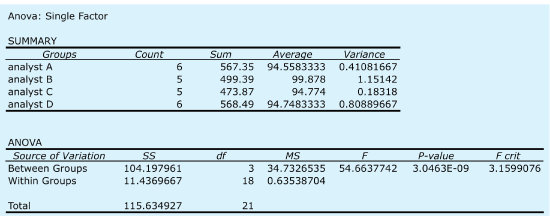
To complete the analysis of variance select Data Analysis... from the Tools menu, which opens a window entitled “Data Analysis.” Scroll through the window, select Analysis: Single Factor from the available options and click OK. Place the cursor in the box for the “Input range” and then click and drag over the cells B1:E7. Select the radio button for “Grouped by: columns” and check the box for “Labels in the first row.” In the box for “Alpha” enter 0.05 for \(\alpha\). Select the radio button for “Output range,” place the cursor in the box and click on an empty cell; this is where Excel will place the results. Clicking OK generates the information shown in Figure \(\PageIndex{2}\). The small value of \(3.05 \times 10^{-9}\) for falsely rejecting the null hypothesis indicates that there is a significant source of variation between the analysts.
R
To complete an analysis of variance for the data in Table 14.3.1 using R, we first need to create several objects. The first object contains each result from Table 14.3.1.
> results = c(94.090, 94.640, 95.008, 94.540, 95.380, 93.620, 99.550, 98.240, 101.100, 100.400, 100.100, 95.140, 94.620, 95.280, 94.590, 94.240, 93.880, 94.230, 96.050, 93.890, 94.950, 95.490)
The second object contains labels that identify the source of each entry in the first object. The following code creates this object.
> analyst = c(rep(“a”,6), rep(“b”,5), rep(“c”,5), rep(“d”,6))
Next, we combine the two objects into a table with two columns, one that contains the data (results) and one that contains the labels (analyst).
> df= data.frame(results, labels= factor(analyst))
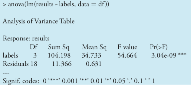
The command factor indicates that the object analyst contains the categorical factors for the analysis of variance. The command for an analysis of variance takes the following form
anova(lm(data ~ factors), data = data.frame)
where data and factors are the columns that contain the data and the categorical factors, and data.frame is the name we assigned to the data table. Figure \(\PageIndex{3}\) shows the resulting output. The small value of \(3.05 \times 10^{-9}\) for falsely rejecting the null hypothesis indicates that there is a significant source of variation between the analysts.
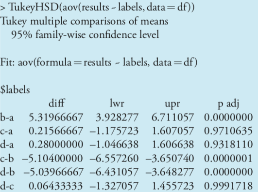
Having found a significant difference between the analysts, we want to identify the source of this difference. R does not include Fisher’s least significant difference test, but it does include a function for a related method called Tukey’s honest significant difference test. The command for this test takes the following form
> TukeyHSD(aov(lm(data ~ factors), data = data.frame), conf. level = 0.5)
where data and factors are the columns that contain the data and the categorical factors, and data.frame is the name we assigned to the data table. Figure \(\PageIndex{4}\) shows the output of this command and its interpretation. The small probability values when comparing analyst B to each of the other analysts indicates that this is the source of the significant difference identified in the analysis of variance.