9.5: Precipitation Titrations

Thus far we have examined titrimetric methods based on acid–base, complexation, and oxidation–reduction reactions. A reaction in which the analyte and titrant form an insoluble precipitate also can serve as the basis for a titration. We call this type of titration a precipitation titration.

One of the earliest precipitation titrations—developed at the end of the eighteenth century—was the analysis of K₂CO₃ and K₂SO₄ in potash. Calcium nitrate, Ca(NO₃)₂, was used as the titrant, which forms a precipitate of CaCO₃ and CaSO₄. The titration’s end point was signaled by noting when the addition of titrant ceased to generate additional precipitate. The importance of precipitation titrimetry as an analytical method reached its zenith in the nineteenth century when several methods were developed for determining Ag⁺ and halide ions.

Titration Curves

A precipitation titration curve follows the change in either the titrand’s or the titrant’s concentration as a function of the titrant’s volume. As we did for other titrations, we first show how to calculate the titration curve and then demonstrate how we can sketch a reasonable approximation of the titration curve.

Calculating the Titration Curve

Let’s calculate the titration curve for the titration of 50.0 mL of 0.0500 M NaCl with 0.100 M AgNO₃. The reaction in this case is

\[\text{Ag}^+(aq) + \text{Cl}^-(aq) \rightleftharpoons \text{AgCl}(s) \nonumber\]

Because the reaction’s equilibrium constant is so large

\[K = (K_\text{sp})^{-1} = (1.8 \times 10^{-10})^{-1} = 5.6 \times 10^9 \nonumber\]

we may assume that Ag⁺ and Cl^– react completely.

By now you are familiar with our approach to calculating a titration curve. The first task is to calculate the volume of Ag⁺ needed to reach the equivalence point. The stoichiometry of the reaction requires that

\[\text{mol Ag}^+ = M_\text{Ag}V_\text{Ag} = M_\text{Cl}V_\text{Cl} = \text{mol Cl}^- \nonumber\]

Solving for the volume of Ag⁺

\[V_{eq} = V_\text{Ag} = \frac{M_\text{Cl}V_\text{Cl}}{M_\text{Ag}} = \frac{(0.0500 \text{ M})(50.0 \text{ mL})}{0.100 \text{ M}} = 25.0 \text{ mL} \nonumber\]

shows that we need 25.0 mL of Ag⁺ to reach the equivalence point.

Before the equivalence point the titrand, Cl^–, is in excess. The concentration of unreacted Cl^– after we add 10.0 mL of Ag⁺, for example, is

\[[\text{Cl}^-] = \frac{(\text{mol Cl}^-)_\text{initial} - (\text{mol Ag}^+)_\text{added}}{\text{total volume}} = \frac{M_\text{Cl}V_\text{Cl} - M_\text{Ag}V_\text{Ag}}{V_\text{Cl} + V_\text{Ag}} \nonumber\]

\[[\text{Cl}^-] = \frac{(0.0500 \text{ M})(50.0 \text{ mL}) - (0.100 \text{ M})(10.0 \text{ mL})}{50.0 \text{ mL} + 10.0 \text{ mL}} = 2.50 \times 10^{-2} \text{ M} \nonumber\]

which corresponds to a pCl of 1.60.

At the titration’s equivalence point, we know that the concentrations of Ag⁺ and Cl^– are equal. To calculate the concentration of Cl^– we use the K_sp for AgCl; thus

\[K_\text{sp} = [\text{Ag}^+][\text{Cl}^-] = (x)(x) = 1.8 \times 10^{-10} \nonumber\]

Solving for x gives [Cl^–] as \(1.3 \times 10^{-5}\) M, or a pCl of 4.89.

After the equivalence point, the titrant is in excess. We first calculate the concentration of excess Ag⁺ and then use the K_sp expression to calculate the concentration of Cl^–. For example, after adding 35.0 mL of titrant

\[[\text{Ag}^+] = \frac{(\text{mol Ag}^+)_\text{added} - (\text{mol Cl}^-)_\text{initial}}{\text{total volume}} = \frac{M_\text{Ag}V_\text{Ag} - M_\text{Cl}V_\text{Cl}}{V_\text{Ag} + V_\text{Cl}} \nonumber\]

\[[\text{Ag}^+] = \frac{(0.100 \text{ M})(35.0 \text{ mL}) - (0.0500 \text{ M})(50.0 \text{ mL})}{35.0 \text{ mL} + 50.0 \text{ mL}} = 1.18 \times 10^{-2} \text{ M} \nonumber\]

\[[\text{Cl}^-] = \frac{K_\text{sp}}{[\text{Ag}^+]} = \frac{1.8 \times 10^{-10}}{1.18 \times 10^{-2}} = 1.5 \times 10^{-8} \text{ M} \nonumber\]

or a pCl of 7.81. Additional results for the titration curve are shown in Table \(\PageIndex{1}\) and Figure \(\PageIndex{1}\).

Table \(\PageIndex{1}\). Titration of 50.0 mL of 0.0500 M NaCl with 0.100 M \(\text{AgNO}_3\)

volume of AgNO3 (mL)	pCl	volume of AgNO3 (mL)	pCl
0.00	1.30	30.0	7.54
5.00	1.44	35.0	7.82
10.0	1.60	40.0	7.97
15.0	1.81	45.0	8.07
20.0	2.15	50.0	8.14
25.0	4.89

Figure \(\PageIndex{1}\). Titration curve for the titration of 50.0 mL of 0.0500 M NaCl with 0.100 M AgNO₃. The red points corresponds to the data in Table \(\PageIndex{1}\). The blue line shows the complete titration curve.

Exercise \(\PageIndex{1}\)

When calculating a precipitation titration curve, you can choose to follow the change in the titrant’s concentration or the change in the titrand’s concentration. Calculate the titration curve for the titration of 50.0 mL of 0.0500 M AgNO₃ with 0.100 M NaCl as pAg versusV_NaCl, and as pCl versus V_NaCl.

Answer

The first task is to calculate the volume of NaCl needed to reach the equivalence point; thus

\[V_{eq} = V_\text{NaCl} = \frac{M_\text{Ag}V_\text{Ag}}{M_\text{NaCl}} = \frac{(0.0500 \text{ M})(50.0 \text{ mL})}{0.100 \text{ M}} = 25.0 \text{ mL} \nonumber\]

Before the equivalence point the titrand, Ag⁺, is in excess. The concentration of unreacted Ag⁺ after adding 10.0 mL of NaCl, for example, is

\[[\text{Ag}^+] = \frac{(0.0500 \text{ M})(50.0 \text{ mL}) - (0.100 \text{ M})(10.0 \text{ mL})}{50.0 \text{ mL} + 10.0 \text{ mL}} = 2.50 \times 10^{-2} \text{ M} \nonumber\]

which corresponds to a pAg of 1.60. To find the concentration of Cl^– we use the K_sp for AgCl; thus

\[[\text{Cl}^-] = \frac{K_\text{sp}}{[\text{Ag}^+]} = \frac{1.8 \times 10^{-10}}{2.50 \times 10^{-2}} = 7.2 \times 10^{-9} \text{ M} \nonumber\]

or a pCl of 8.14.

At the titration’s equivalence point, we know that the concentrations of Ag⁺ and Cl^– are equal. To calculate their concentrations we use the Ksp expression for AgCl; thus

\[K_\text{sp} = [\text{Ag}^+][\text{Cl}^-] = (x)(x) = 1.8 \times 10^{-10} \nonumber\]

Solving for x gives the concentration of Ag⁺ and the concentration of Cl^– as \(1.3 \times 10^{-5}\) M, or a pAg and a pCl of 4.89.

After the equivalence point, the titrant is in excess. For example, after adding 35.0 mL of titrant

\[[\text{Cl}^-] = \frac{(0.100 \text{ M})(35.0 \text{ mL}) - (0.0500 \text{ M})(50.0 \text{ mL})}{35.0 \text{ mL} + 50.0 \text{ mL}} = 1.18 \times 10^{-2} \text{ M} \nonumber\]

or a pCl of 1.93. To find the concentration of Ag⁺ we use the K_sp for AgCl; thus

\[[\text{Ag}^+] = \frac{K_\text{sp}}{[\text{Cl}^-]} = \frac{1.8 \times 10^{-10}}{1.18 \times 10^{-2}} = 1.5 \times 10^{-8} \text{ M} \nonumber\]

or a pAg of 7.82. The following table summarizes additional results for this titration.

volume of NaCl (mL)	pAg	pCl
0	1.30	—
5.00	1.44	8.31
10.0	1.60	8.14
15.0	1.81	7.93
20.0	2.15	7.60
25.0	4.89	4.89
30.0	7.54	2.20
35.0	7.82	1.93
40.0	7.97	1.78
45.0	8.07	1.68
50.0	8.14	1.60

Sketching the Titration Curve

To evaluate the relationship between a titration’s equivalence point and its end point we need to construct only a reasonable approximation of the exact titration curve. In this section we demonstrate a simple method for sketching a precipitation titration curve. Our goal is to sketch the titration curve quickly, using as few calculations as possible. Let’s use the titration of 50.0 mL of 0.0500 M NaCl with 0.100 M AgNO₃.

This is the same example that we used in developing the calculations for a precipitation titration curve. You can review the results of that calculation in Table \(\PageIndex{1}\) and Figure \(\PageIndex{1}\).

We begin by calculating the titration’s equivalence point volume, which, as we determined earlier, is 25.0 mL. Next we draw our axes, placing pCl on the y-axis and the titrant’s volume on the x-axis. To indicate the equivalence point’s volume, we draw a vertical line that intersects the x-axis at 25.0 mL of AgNO₃. Figure \(\PageIndex{2}\)a shows the result of this first step in our sketch.

Figure \(\PageIndex{2}\). Illustrations showing the steps in sketching an approximate titration curve for the titration of 50.0 mL of 0.0500 M NaCl with 0.100 M AgNO₃: (a) locating the equivalence point volume; (b) plotting two points before the equivalence point; (c) plotting two points after the equivalence point; (d) preliminary approximation of titration curve using straight-lines; (e) final approximation of titration curve using a smooth curve; (f) comparison of approximate titration curve (solid black line) and exact titration curve (dashed red line). See the text for additional details. A better fit is possible if the two points before the equivalence point are further apart—for example, 0 mL and 20 mL—and the two points after the equivalence point are further apart.

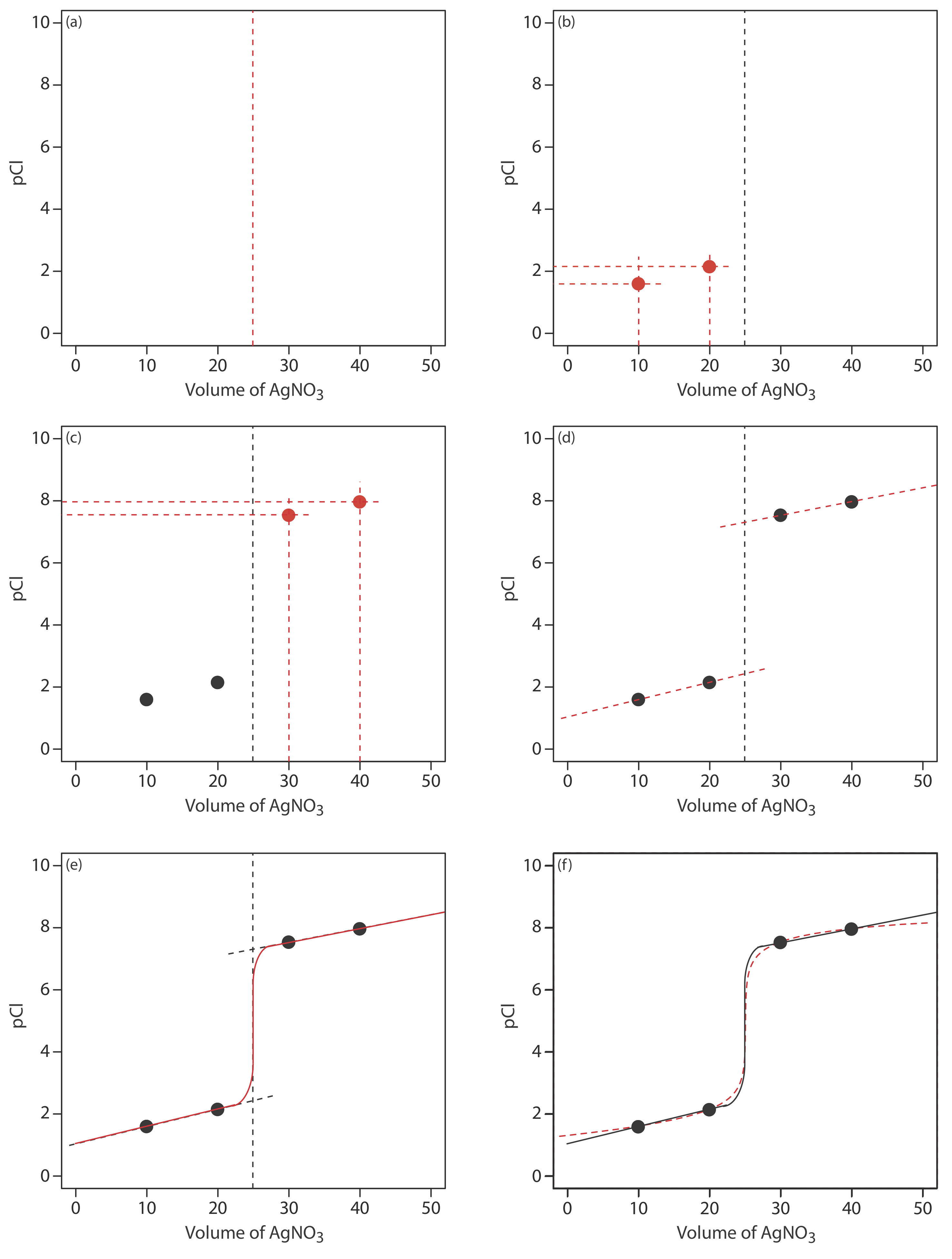
Before the equivalence point, Cl^– is present in excess and pCl is determined by the concentration of unreacted Cl^–. As we learned earlier, the calculations are straightforward. Figure \(\PageIndex{2}\)b shows pCl after adding 10.0 mL and 20.0 mL of AgNO₃.

After the equivalence point, Ag⁺ is in excess and the concentration of Cl^– is determined by the solubility of AgCl. Again, the calculations are straightforward. Figure \(\PageIndex{2}\)c shows pCl after adding 30.0 mL and 40.0 mL of AgNO₃.

Next, we draw a straight line through each pair of points, extending them through the vertical line that represents the equivalence point’s volume (Figure \(\PageIndex{2}\)d). Finally, we complete our sketch by drawing a smooth curve that connects the three straight-line segments (Figure \(\PageIndex{2}\)e). A comparison of our sketch to the exact titration curve (Figure \(\PageIndex{2}\)f) shows that they are in close agreement.

Selecting and Evaluating the End Point

At the beginning of this section we noted that the first precipitation titration used the cessation of precipitation to signal the end point. At best, this is a cumbersome method for detecting a titration’s end point. Before precipitation titrimetry became practical, better methods for identifying the end point were necessary.

Finding the End Point With an Indicator

There are three general types of indicators for a precipitation titration, each of which changes color at or near the titration’s equivalence point. The first type of indicator is a species that forms a precipitate with the titrant. In the Mohr method for Cl^– using Ag⁺ as a titrant, for example, a small amount of K₂CrO₄ is added to the titrand’s solution. The titration’s end point is the formation of a reddish-brown precipitate of Ag₂CrO₄.

The Mohr method was first published in 1855 by Karl Friedrich Mohr.

Because \(\text{CrO}_4^{2-}\) imparts a yellow color to the solution, which might obscure the end point, only a small amount of K₂CrO₄ is added. As a result, the end point is always later than the equivalence point. To compensate for this positive determinate error, an analyte-free reagent blank is analyzed to determine the volume of titrant needed to affect a change in the indicator’s color. Subtracting the end point for the reagent blank from the titrand’s end point gives the titration’s end point. Because \(\text{CrO}_4^{2-}\) is a weak base, the titrand’s solution is made slightly alkaline. If the pH is too acidic, chromate is present as \(\text{HCrO}_4^{-}\) instead of \(\text{CrO}_4^{2-}\), and the Ag₂CrO₄ end point is delayed. The pH also must be less than 10 to avoid the precipitation of silver hydroxide.

A second type of indicator uses a species that forms a colored complex with the titrant or the titrand. In the Volhard method for Ag⁺ using KSCN as the titrant, for example, a small amount of Fe³⁺ is added to the titrand’s solution. The titration’s end point is the formation of the reddish-colored Fe(SCN)²⁺ complex. The titration is carried out in an acidic solution to prevent the precipitation of Fe³⁺ as Fe(OH)₃.

The Volhard method was first published in 1874 by Jacob Volhard.

The third type of end point uses a species that changes color when it adsorbs to the precipitate. In the Fajans method for Cl^– using Ag⁺ as a titrant, for example, the anionic dye dichlorofluoroscein is added to the titrand’s solution. Before the end point, the precipitate of AgCl has a negative surface charge due to the adsorption of excess Cl^–. Because dichlorofluoroscein also carries a negative charge, it is repelled by the precipitate and remains in solution where it has a greenish-yellow color. After the end point, the surface of the precipitate carries a positive surface charge due to the adsorption of excess Ag⁺. Dichlorofluoroscein now adsorbs to the precipitate’s surface where its color is pink. This change in the indicator’s color signals the end point.

The Fajans method was first published in the 1920s by Kasimir Fajans.

Finding the End Point Potentiometrically

Another method for locating the end point is a potentiometric titration in which we monitor the change in the titrant’s or the titrand’s concentration using an ion-selective electrode. The end point is found by visually examining the titration curve. For a discussion of potentiometry and ion-selective electrodes, see Chapter 11.

Quantitative Applications

Although precipitation titrimetry rarely is listed as a standard method of analysis, it is useful as a secondary analytical method to verify other analytical methods. Most precipitation titrations use Ag⁺ as either the titrand or the titrant. A titration in which Ag⁺ is the titrant is called an argentometric titration. Table \(\PageIndex{2}\) provides a list of several typical precipitation titrations.

Table \(\PageIndex{2}\). Representative Examples of Precipitation Titrations

titrand	titrant	end point
\(\text{AsO}_4^{3-}\)	AgNO3 and KSCN	Volhard
Br^–	AgNO3 AgNO3 and KSCN	Mohr or Fajans Volhard
Cl^–	AgNO3 AgNO3 and KSCN	Mohr or Fajarns Volhard^*
\(\text{CO}_3^-\)	AgNO3 and KSCN	Volhard^*
\(\text{C}_2\text{O}_4^{2-}\)	AgNO3 and KSCN	Volhard^*
\(\text{CrO}_4^{2-}\)	AgNO3 and KSCN	Volhard^*
I^–	AgNO3 AgNO3 and KSCN	Fajans Volhard
\(\text{PO}_4^{3-}\)	AgNO3 and KSCN	Volhard^*
S^2–	AgNO3 and KSCN	Volhard^*
SCN^–	AgNO3 and KSCN	Volhard^*
When two titrants are listed (AgNO3 and KSCN), the analysis is by a back titration; the first titrant, AgNO3, is added in excess and the excess is titrated using the second titrant, KSCN. For those Volhard methods identified with an asterisk (*), the precipitated silver salt is removed before carrying out the back titration.

Quantitative Calculations

The quantitative relationship between the titrand and the titrant is determined by the stoichiometry of the titration reaction. If you are unsure of the balanced reaction, you can deduce the stoichiometry from the precipitate’s formula. For example, in forming a precipitate of Ag₂CrO₄, each mole of \(\text{CrO}_4^{2-}\) reacts with two moles of Ag⁺.

Example \(\PageIndex{1}\)

A mixture containing only KCl and NaBr is analyzed by the Mohr method. A 0.3172-g sample is dissolved in 50 mL of water and titrated to the Ag₂CrO₄ end point, requiring 36.85 mL of 0.1120 M AgNO₃. A blank titration requires 0.71 mL of titrant to reach the same end point. Report the %w/w KCl in the sample.

Solution

To find the moles of titrant reacting with the sample, we first need to correct for the reagent blank; thus

\[V_\text{Ag} = 36.85 \text{ mL} - 0.71 \text{ mL} = 36.14 \text{ mL} \nonumber\]

\[(0.1120 \text{ M})(0.03614 \text{ L}) = 4.048 \times 10^{-3} \text{ mol AgNO}_3 \nonumber\]

Titrating with AgNO₃ produces a precipitate of AgCl and AgBr. In forming the precipitates, each mole of KCl consumes one mole of AgNO₃ and each mole of NaBr consumes one mole of AgNO₃; thus

\[\text{mol KCl + mol NaBr} = 4.048 \times 10^{-3} \text{ mol AgNO}_3 \nonumber\]

We are interested in finding the mass of KCl, so let’s rewrite this equation in terms of mass. We know that

\[\text{mol KCl} = \frac{\text{g KCl}}{74.551 \text{g KCl/mol KCl}} \nonumber\]

\[\text{mol NaBr} = \frac{\text{g NaBr}}{102.89 \text{g NaBr/mol NaBr}} \nonumber\]

which we substitute back into the previous equation

\[\frac{\text{g KCl}}{74.551 \text{g KCl/mol KCl}} + \frac{\text{g NaBr}}{102.89 \text{g NaBr/mol NaBr}} = 4.048 \times 10^{-3} \nonumber\]

Because this equation has two unknowns—g KCl and g NaBr—we need another equation that includes both unknowns. A simple equation takes advantage of the fact that the sample contains only KCl and NaBr; thus,

\[\text{g NaBr} = 0.3172 \text{ g} - \text{ g KCl} \nonumber\]

\[\frac{\text{g KCl}}{74.551 \text{g KCl/mol KCl}} + \frac{0.3172 \text{ g} - \text{ g KCl}}{102.89 \text{g NaBr/mol NaBr}} = 4.048 \times 10^{-3} \nonumber\]

\[1.341 \times 10^{-2}(\text{g KCl}) + 3.083 \times 10^{-3} - 9.719 \times 10^{-3} (\text{g KCl}) = 4.048 \times 10^{-3} \nonumber\]

\[3.69 \times 10^{-3}(\text{g KCl}) = 9.65 \times 10^{-4} \nonumber\]

The sample contains 0.262 g of KCl and the %w/w KCl in the sample is

\[\frac{0.262 \text{ g KCl}}{0.3172 \text{ g sample}} \times 100 = 82.6 \text{% w/w KCl} \nonumber\]

The analysis for I^– using the Volhard method requires a back titration. A typical calculation is shown in the following example.

Example \(\PageIndex{2}\)

The %w/w I^– in a 0.6712-g sample is determined by a Volhard titration. After adding 50.00 mL of 0.05619 M AgNO₃ and allowing the precipitate to form, the remaining silver is back titrated with 0.05322 M KSCN, requiring 35.14 mL to reach the end point. Report the %w/w I^– in the sample.

Solution

There are two precipitates in this analysis: AgNO₃ and I^– form a precipitate of AgI, and AgNO₃ and KSCN form a precipitate of AgSCN. Each mole of I^– consumes one mole of AgNO₃ and each mole of KSCN consumes one mole of AgNO₃; thus

\[\text{mol AgNO}_3 = \text{mol I}^- + \text{mol KSCN} \nonumber\]

Solving for the moles of I^– we find

\[\text{mol I}^- = \text{mol AgNO}_3 - \text{mol KSCN} = M_\text{Ag} V_\text{Ag} - M_\text{KSCN} V_\text{KSCN} \nonumber\]

\[\text{mol I}^- = (0.05619 \text{ M})(0.0500 \text{ L}) - (0.05322 \text{ M})(0.03514 \text{ L}) = 9.393 \times 10^{-4} \nonumber\]

The %w/w I^– in the sample is

\[\frac{(9.393 \times 10^{-4} \text{ mol I}^-) \times \frac{126.9 \text{ g I}^-}{\text{mol I}^-}}{0.6712 \text{ g sample}} \times 100 = 17.76 \text{% w/w I}^- \nonumber\]

Exercise \(\PageIndex{2}\)

A 1.963-g sample of an alloy is dissolved in HNO₃ and diluted to volume in a 100-mL volumetric flask. Titrating a 25.00-mL portion with 0.1078 M KSCN requires 27.19 mL to reach the end point. Calculate the %w/w Ag in the alloy.

Answer

The titration uses

\[(0.1078 \text{ M KSCN})(0.02719 \text{ L}) = 2.931 \times 10^{-3} \text{ mol KSCN} \nonumber\]

The stoichiometry between SCN^– and Ag⁺ is 1:1; thus, there are

\[2.931 \times 10^{-3} \text{ mol Ag}^+ \times \frac{107.87 \text{ g Ag}}{\text{mol Ag}} = 0.3162 \text{ g Ag} \nonumber\]

in the 25.00 mL sample. Because this represents 1⁄4 of the total solution, there are \(0.3162 \times 4\) or 1.265 g Ag in the alloy. The %w/w Ag in the alloy is

\[\frac{1.265 \text{ g Ag}}{1.963 \text{ g sample}} \times 100 = 64.44 \text{% w/w Ag} \nonumber\]

Evaluation of Precipitation Titrimetry

The scale of operations, accuracy, precision, sensitivity, time, and cost of a precipitation titration is similar to those described elsewhere in this chapter for acid–base, complexation, and redox titrations. Precipitation titrations also can be extended to the analysis of mixtures provided there is a significant difference in the solubilities of the precipitates. Figure \(\PageIndex{3}\) shows an example of a titration curve for a mixture of I^– and Cl^– using Ag⁺ as a titrant.

Figure \(\PageIndex{3}\). Titration curve for the titration of a 50.0 mL mixture of 0.0500 M I^– and 0.0500 M Cl^– using 0.100 M Ag⁺ as a titrant. The red arrows show the end points. Note that the end point for I^– is earlier than the end point for Cl^– because AgI is less soluble than AgCl.