7.4: Solving Titration Problems

Skills to Develop

• Calculate the pH at any point in an acid–base titration.

In this section, we will see how to perform calculations to predict the pH at any point in a titration of a weak acid or base, using the techniques we already know for acid-base equilibria and buffers. 

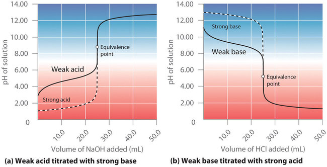
Consider Figure \(\PageIndex{1}\) from the previous section, showing the curves for the titrations of a weak acid or weak base. The pH at different points in each curve is determined by what species are present in the mixture at that point. Thus, we must use different techniques to solve for the pH depending on how far along the titration is. There are three scenarios we will consider, using the titration of 50.0 mL of 0.100 M acetic acid with 0.200 M NaOH (Figure \(\PageIndex{1a}\)) as an example: 

• The pH at the beginning of the titration, before any titrant is added
• The pH in the buffer region, before reaching the equivalence point
• The pH at the equivalence point

In the following examples, we will use a \(pK_a\) of 4.76 for acetic acid at 25°C (\(K_a = 1.7 \times 10^{-5}\)).

Figure \(\PageIndex{3}\): The Titration of (a) a Weak Acid with a Strong Base and (b) a Weak Base with a Strong Acid. (a) As 0.200 M \(NaOH\) is slowly added to 50.0 mL of 0.100 M acetic acid, the pH increases slowly at first, then increases rapidly as the equivalence point is approached, and then again increases more slowly. The corresponding curve for the titration of 50.0 mL of 0.100 M HCl with 0.200 M \(NaOH\) is shown as a dashed line. (b) As 0.200 M HCl is slowly added to 50.0 mL of 0.100 M NH₃, the pH decreases slowly at first, then decreases rapidly as the equivalence point is approached, and then again decreases more slowly. The corresponding curve for the titration of 50.0 mL of 0.100 M \(NaOH\) with 0.200 M HCl is shown as a dashed line.

Calculating the pH of a Solution of a Weak Acid or a Weak Base

At the beginning of a titration, we simply have a solution of a weak acid or base of a certain concentration. As discussed in the previous chapter, if we know \(K_a\) or \(K_b\) and the initial concentration of a weak acid or a weak base, we can calculate the pH by setting up an ICE table (i.e, initial concentrations, changes in concentrations, and equilibrium concentrations). In this situation, the initial concentration of acetic acid is 0.100 M. If we define \(x\) as \([\ce{H^{+}}]\) due to the dissociation of the acid, then the table of concentrations for the ionization of 0.100 M acetic acid is as follows:

\[CH_3CO_2H_{(aq)} \rightleftharpoons H^+_{(aq)} + CH_3CO_2^−\]

ICE	\([CH_3CO_2H]\)	\([H^+]\)	\([CH_3CO_2^−]\)
initial	0.100	\(1.00 \times 10^{−7}\)	0
change	−x	+x	+x
equilibrium	0.100 − x	x	x

In this and all subsequent examples, we will ignore \([H^+]\) and \([OH^-]\) due to the autoionization of water when calculating the final concentration. (However, you should check that this assumption is justified!)

Inserting the expressions for the final concentrations into the equilibrium equation (and using approximations),

\[K_a=\dfrac{[H^+][CH_3CO_2^-]}{[CH_3CO_2H]}=\dfrac{(x)(x)}{0.100 - x} \approx \dfrac{x^2}{0.100}=1.74 \times 10^{-5}\]

Solving this equation gives \(x = [H^+] = 1.32 \times 10^{-3}\; M\). Thus the pH of a 0.100 M solution of acetic acid is as follows:

\[pH = −\log(1.32 \times 10^{-3}) = 2.879\]

Calculating the pH during the Titration of a Weak Acid or a Weak Base

Now consider what happens when we begin to add \(NaOH\) to the \(CH_3CO_2H\) (Figure \(\PageIndex{1a}\)). Because the neutralization reaction with strong base proceeds to completion, all of the \(OH^-\) ions added will react with the acetic acid to generate acetate ion and water:

\[ CH_3CO_2H_{(aq)} + OH^-_{(aq)} \rightarrow CH_3CO^-_{2\;(aq)} + H_2O_{(l)} \label{Eq2}\]

All problems of this type must be solved in two steps: a stoichiometric calculation followed by an equilibrium calculation. In the first step, we use the stoichiometry of the neutralization reaction to calculate the amounts of acid and conjugate base present in solution after the neutralization reaction has occurred. In the second step, we use the equilibrium equation to determine \([\ce{H^{+}}]\) of the resulting solution. 

Example \(\PageIndex{1}\): Calculating pH in the Buffer Region

What is the pH when 5.00 mL of 0.200 M \(NaOH\) has been added to 50.00 mL of 0.100 M \(CH_3CO_2H\) (part (a) in Figure \(\PageIndex{1}\))? 

Strategy

Step 1: Use stoichiometry of the neutralization to determine the amounts of acid and conjugate base present in solution

Step 2: Solve for equilibrium concentrations using ICE tables or Henderson-Hasselbalch approximation

Solution

Step 1

To determine the amount of acid and conjugate base in solution after the neutralization reaction, we calculate the amount of \(\ce{CH_3CO_2H}\) in the original solution and the amount of \(\ce{OH^{-}}\) in the \(\ce{NaOH}\) solution that was added. The acetic acid solution contained

\[ 50.00 \; \cancel{mL} (0.100 \;mmol (\ce{CH_3CO_2H})/\cancel{mL} )=5.00\; mmol (\ce{CH_3CO_2H}) \]

The \(\ce{NaOH}\) solution contained

5.00 mL=1.00 mmol \(NaOH\)

Comparing the amounts shows that \(CH_3CO_2H\) is in excess. Because \(OH^-\) reacts with \(CH_3CO_2H\) in a 1:1 stoichiometry, the amount of excess \(CH_3CO_2H\) is as follows:

5.00 mmol \(CH_3CO_2H\) − 1.00 mmol \(OH^-\) = 4.00 mmol \(CH_3CO_2H\)

Each 1 mmol of \(OH^-\) reacts to produce 1 mmol of acetate ion, so the final amount of \(CH_3CO_2^−\) is 1.00 mmol.

The stoichiometry of the reaction is summarized in the following table, which shows the numbers of moles of the various species, not their concentrations.

\[\ce{CH3CO2H(aq) + OH^{−} (aq) <=> CH3CO2^{-}(aq) + H2O(l)}\]

ICE	\([\ce{CH_3CO_2H}]\)	\([\ce{OH^{−}}]\)	\([\ce{CH_3CO_2^{−}}]\)
initial	5.00 mmol	1.00 mmol	0 mmol
change	−1.00 mmol	−1.00 mmol	+1.00 mmol
final	4.00 mmol	0 mmol	1.00 mmol

This ICE table gives the initial amount of acetate and the final amount of \(OH^-\) ions as 0. Because an aqueous solution of acetic acid always contains at least a small amount of acetate ion in equilibrium with acetic acid, the initial acetate concentration is not actually 0. The value can be ignored in this calculation, however, because the amount of \(CH_3CO_2^−\) in equilibrium is insignificant compared to the amount of \(OH^-\) added. Moreover, due to the autoionization of water, no aqueous solution can contain 0 mmol of \(OH^-\), but the amount of \(OH^-\) due to the autoionization of water is insignificant compared to the amount of \(OH^-\) added. We use the initial amounts of the reactants to determine the stoichiometry of the reaction and defer a consideration of the equilibrium until the second half of the problem.

Step 2

Now that we have determined that there is a mixture of \(\ce{CH_3CO_2H}\) and \(\ce{CH3CO2^{−}}\) present in solution, we know that this point in the titration is in the buffer region. Therefore, we can use the equilibrium method or the Henderson-Hasselbalch equation. 

To calculate \([\ce{H^{+}}]\) using the acid ionization equilibrium, we must first calculate [\(\ce{CH_3CO_2H}\)] and \([\ce{CH3CO2^{−}}]\) using the number of millimoles of each and the total volume of the solution at this point in the titration:

\[ final \;volume=50.00 \;mL+5.00 \;mL=55.00 \;mL \] \[ \left [ CH_{3}CO_{2}H \right ] = \dfrac{4.00 \; mmol \; CH_{3}CO_{2}H }{55.00 \; mL} =7.27 \times 10^{-2} \;M \] \[ \left [ CH_{3}CO_{2}^{-} \right ] = \dfrac{1.00 \; mmol \; CH_{3}CO_{2}^{-} }{55.00 \; mL} =1.82 \times 10^{-2} \;M \]

Knowing the concentrations of acetic acid and acetate ion at equilibrium and \(K_a\) for acetic acid (\(1.74 \times 10^{-5}\)), we can calculate \([H^+]\) at equilibrium:

\[ K_{a}=\dfrac{\left [ CH_{3}CO_{2}^{-} \right ]\left [ H^{+} \right ]}{\left [ CH_{3}CO_{2}H \right ]} \]

\[ \left [ H^{+} \right ]=\dfrac{K_{a}\left [ CH_{3}CO_{2}H \right ]}{\left [ CH_{3}CO_{2}^{-} \right ]} = \dfrac{\left ( 1.72 \times 10^{-5} \right )\left ( 7.27 \times 10^{-2} \;M\right )}{\left ( 1.82 \times 10^{-2} \right )}= 6.95 \times 10^{-5} \;M \]

Calculating \(−\log[\ce{H^{+}}]\) gives

\[pH = −\log(6.95 \times 10^{−5}) = 4.158.\]

Alternatively, since the concentrations of each component are large compared to \(K_a\), we can use the Henderson-Hasselbalch approximation, treating the system as a buffer: 

\[pH=pK_a+\log \left( \dfrac{[A^−]}{[HA]} \right)\]

\[pH= 4.76+\log \left( \dfrac{1.00 mmol}{4.00 mmol} = 4.76 + (-0.602) = 4.158 \right)\]

This approach is mathematically equivalent to the first, but note that it is not necessary to convert millimoles into molar concentration to use the Henderson-Hasselbalch equation, which makes this method a little simpler. 

Exercise \(\PageIndex{1}\)

Calculate the pH of a solution prepared by adding 45.0 mL of a 0.213 M HCl solution to 125.0 mL of a 0.150 M solution of ammonia. The \(pK_b\) of ammonia is 4.75 at 25°C.

Answer

9.23 (Note that since the ammonia is approximately half-neutralized at this point, this pH is very close to the \(pK_a\) of ammonium, 9.25!)

Any pH point in a titration before the weak acid is fully neutralized can be solved by the above method. At the equivalence point, however, there is no longer a significant amount of the starting acid remaining, and the sample no longer constitutes a buffer. Rather, the sample consists predominantly of the weak acid's conjugate base. The pH is determined by this base's concentration and \(pK_b\), and can be solved for using a base dissociation equilibrium. In Example \(\PageIndex{2}\), we calculate the pH at the equivalence point of our titration curve of acetic acid.

Example \(\PageIndex{2}\): Calculating pH at the Equivalence Point

What is the pH of the solution after 25.00 mL of 0.200 M \(NaOH\) is added to 50.00 mL of 0.100 M acetic acid?

Given: volume and molarity of base and acid

Asked for: pH

Strategy:

1. Write the balanced chemical equation for the reaction. Then calculate the initial numbers of millimoles of \(OH^-\) and \(CH_3CO_2H\). Determine which species, if either, is present in excess.
2. Tabulate the results showing initial numbers, changes, and final numbers of millimoles.
3. If excess acetate is present after the reaction with \(OH-\), write the equation for the reaction of acetate with water. Use a tabular format to obtain the concentrations of all the species present.
4. Calculate \(K_b\) using the relationship \(K_w = K_aK_b\). Calculate [OH−] and use this to calculate the pH of the solution.

SOLUTION

A Ignoring the spectator ion (\(Na^+\)), the equation for this reaction is as follows:

\[CH_3CO_2H_{ (aq)} + OH^-(aq) \rightarrow CH_3CO_2^-(aq) + H_2O(l) \]

The initial numbers of millimoles of \(OH^-\) and \(CH_3CO_2H\) are as follows:

25.00 mL(0.200 mmol \(OH-\)/mL)=5.00 mmol \(OH-\)

\[50.00\; mL (0.100 mmol CH_3CO_2 H/mL)=5.00 mmol \; CH_3CO_2H \]

The number of millimoles of \(OH^-\) equals the number of millimoles of \(CH_3CO_2H\), so neither species is present in excess.

B Because the number of millimoles of \(OH^-\) added corresponds to the number of millimoles of acetic acid in solution, this is the equivalence point. The results of the neutralization reaction can be summarized in tabular form.

\[CH_3CO_2H_{(aq)}+OH^-_{(aq)} \rightleftharpoons CH_3CO_2^{-}(aq)+H_2O(l) \]

ICE	\([\ce{CH3CO2H}]\)	\([\ce{OH^{−}}]\)	\([\ce{CH3CO2^{−}}]\)
initial	5.00 mmol	5.00 mmol	0 mmol
change	−5.00 mmol	−5.00 mmol	+5.00 mmol
final	0 mmol	0 mmol	5.00 mmol

C Because the product of the neutralization reaction is a weak base, we must consider the reaction of the weak base with water to calculate [H+] at equilibrium and thus the final pH of the solution. The initial concentration of acetate is obtained from the neutralization reaction:

\[ [\ce{CH_3CO_2}]=\dfrac{5.00 \;mmol \; CH_3CO_2^{-}}{(50.00+25.00) \; mL}=6.67\times 10^{-2} \; M \]

The equilibrium reaction of acetate with water is as follows:

\[\ce{CH_3CO^{-}2(aq) + H2O(l) <=> CH3CO2H(aq) + OH^{-} (aq)} \]

The equilibrium constant for this reaction is

\[K_b = \dfrac{K_w}{K_a} \label{16.18}\]

where \(K_a\) is the acid ionization constant of acetic acid. We therefore define x as \([\ce{OH^{−}}]\) produced by the reaction of acetate with water. Here is the completed table of concentrations:

\[H_2O_{(l)}+CH_3CO^−_{2(aq)} \rightleftharpoons CH_3CO_2H_{(aq)} +OH^−_{(aq)} \]

	\([\ce{CH3CO2^{−}}]\)	\([\ce{CH3CO2H}]\)	\([\ce{OH^{−}}]\)
initial	0.0667	0	1.00 × 10−7
change	−x	+x	+x
equilibrium	(0.0667 − x)	x	x

D Substituting the expressions for the final values from this table into Equation \ref{16.18},

\[ K_{b}= \dfrac{K_w}{K_a} =\dfrac{1.01 \times 10^{-14}}{1.74 \times 10^{-5}} = 5.80 \times 10^{-10}=\dfrac{x^{2}}{0.0667} \label{16.23}\]

We can obtain \(K_b\) by rearranging Equation \ref{16.23} and substituting the known values:

\[K_b=K_wK_a=(1.01×10^{−14})(1.74×10^{−5})=5.80×10^{−10}=x20.0667 \]

which we can solve to get \(x = 6.22 \times 10^{−6}\). Thus \([OH^{−}] = 6.22 \times 10^{−6}\, M\), and the pH of the final solution is 8.794 (Figure \(\PageIndex{3a}\)). As expected for the titration of a weak acid, the pH at the equivalence point is greater than 7.00 because the product of the titration is a base, the acetate ion, which then reacts with water to produce \(\ce{OH^{-}}\).

Exercise \(\PageIndex{2}\)

Calculate the pH of a solution prepared by adding 88.0 mL of a 0.213 M HCl solution to 125.0 mL of a 0.150 M solution of ammonia. The \(pK_b\) of ammonia is 4.75 at 25°C.

Answer

5.14

Titrations of Polyprotic Acids or Bases

When a strong base is added to a solution of a polyprotic acid, the neutralization reaction occurs in stages. The most acidic group is titrated first, followed by the next most acidic, and so forth. If the \(pK_a\) values are separated by at least three \(pK_a\) units, then the overall titration curve shows well-resolved “steps” corresponding to the titration of each proton. A titration of the triprotic acid \(H_3PO_4\) with \(NaOH\) is illustrated in Figure \(\PageIndex{2}\) and shows two well-defined steps: the first midpoint corresponds to \(pK_a\)1, and the second midpoint corresponds to \(pK_a\)₂. Because HPO₄²⁻ is such a weak acid, \(pK_a\)₃ has such a high value that the third step cannot be resolved using 0.100 M \(NaOH\) as the titrant.

Figure \(\PageIndex{2}\): Titration Curve for Phosphoric Acid (\(H_3PO_4\), a Typical Polyprotic Acid. The curve for the titration of 25.0 mL of a 0.100 M \(H_3PO_4\) solution with 0.100 M \(NaOH\) along with the species in solution at each Ka is shown. Note the two distinct equivalence points corresponding to deprotonation of \(H_3PO_4\) at pH ≈ 4.6 and \(H_2PO_4^{2-}\) at pH ≈ 9.8. Because \(HPO_4^{2−}\) is a very weak acid, the third equivalence point, at pH ≈ 13, is not well defined.

The titration curve for the reaction of a polyprotic base with a strong acid is the mirror image of the curve shown in Figure \(\PageIndex{2}\). The initial pH is high, but as acid is added, the pH decreases in steps if the successive \(pK_b\) values are well separated. 

In calculating the pH in a titration of a polyprotic acid or base, it is important to know which \(pK_a\) or \(pK_b\) value to use, based on the reaction stoichiometry at the point of interest.

Example \(\PageIndex{3}\)

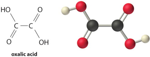
Calculate the pH of a solution prepared by adding 55.0 mL of a 0.120 M \(NaOH\) solution to 100.0 mL of a 0.0510 M solution of oxalic acid (\(HO_2CCO_2\)H), a diprotic acid (abbreviated as H2ox). Oxalic acid, the simplest dicarboxylic acid, is found in rhubarb and many other plants. Rhubarb leaves are toxic because they contain the calcium salt of the fully deprotonated form of oxalic acid, the oxalate ion (−O₂CCO²⁻, abbreviated \(ox^{2-}\)). Oxalate salts are toxic for two reasons. First, oxalate salts of divalent cations such as \(Ca^{2+}\) are insoluble at neutral pH but soluble at low pH. As a result, calcium oxalate dissolves in the dilute acid of the stomach, allowing oxalate to be absorbed and transported into cells, where it can react with calcium to form tiny calcium oxalate crystals that damage tissues. Second, oxalate forms stable complexes with metal ions, which can alter the distribution of metal ions in biological fluids.

Given: volume and concentration of acid and base

Asked for: pH

Strategy:

1. Calculate the initial millimoles of the acid and the base. Use a tabular format to determine the amounts of all the species in solution.
2. Calculate the concentrations of all the species in the final solution. Determine \(\ce{[H{+}]}\) and convert this value to pH.

Solution:

A Table E5 gives the \(pK_a\) values of oxalic acid as 1.25 and 3.81. Again we proceed by determining the millimoles of acid and base initially present:

\[ 100.00 \cancel{mL} \left ( \dfrac{0.510 \;mmol \;H_{2}ox}{\cancel{mL}} \right )= 5.10 \;mmol \;H_{2}ox \]

\[ 55.00 \cancel{mL} \left ( \dfrac{0.120 \;mmol \;NaOH}{\cancel{mL}} \right )= 6.60 \;mmol \;NaOH \]

The strongest acid (\(H_2ox\)) reacts with the base first. This leaves (6.60 − 5.10) = 1.50 mmol of \(OH^-\) to react with Hox−, forming ox²⁻ and H₂O. The reactions can be written as follows:

\[ \underset{5.10\;mmol}{H_{2}ox}+\underset{6.60\;mmol}{OH^{-}} \rightarrow \underset{5.10\;mmol}{Hox^{-}}+ \underset{5.10\;mmol}{H_{2}O} \]

\[ \underset{5.10\;mmol}{Hox^{-}}+\underset{1.50\;mmol}{OH^{-}} \rightarrow \underset{1.50\;mmol}{ox^{2-}}+ \underset{1.50\;mmol}{H_{2}O} \]

In tabular form,

	\(\ce{H2ox}\)	\(\ce{OH^{-}}\)	\(\ce{Hox^{−}}\)	\(\ce{ox^{2−}}\)
initial	5.10 mmol	6.60 mmol	0 mmol	0 mmol
change (step 1)	−5.10 mmol	−5.10 mmol	+5.10 mmol	0 mmol
final (step 1)	0 mmol	1.50 mmol	5.10 mmol	0 mmol
change (step 2)	—	−1.50 mmol	−1.50 mmol	+1.50 mmol
final	0 mmol	0 mmol	3.60 mmol	1.50 mmol

B The equilibrium between the weak acid (\(\ce{Hox^{-}}\)) and its conjugate base (\(\ce{ox^{2-}}\)) in the final solution is determined by the magnitude of the second ionization constant, \(K_{a2} = 10^{−3.81} = 1.6 \times 10^{−4}\). To calculate the pH of the solution, we need to know \(\ce{[H^{+}]}\), which is determined using exactly the same method as in the acetic acid titration in Example \(\PageIndex{2}\):

final volume of solution = 100.0 mL + 55.0 mL = 155.0 mL

Thus the concentrations of \(\ce{Hox^{-}}\) and \(\ce{ox^{2-}}\) are as follows:

\[ \left [ Hox^{-} \right ] = \dfrac{3.60 \; mmol \; Hox^{-}}{155.0 \; mL} = 2.32 \times 10^{-2} \;M \]

\[ \left [ ox^{2-} \right ] = \dfrac{1.50 \; mmol \; ox^{2-}}{155.0 \; mL} = 9.68 \times 10^{-3} \;M \]

We can now calculate [H+] at equilibrium using the following equation:

\[ K_{a2} =\dfrac{\left [ ox^{2-} \right ]\left [ H^{+} \right ] }{\left [ Hox^{-} \right ]} \]

Rearranging this equation and substituting the values for the concentrations of \(\ce{Hox^{−}}\) and \(\ce{ox^{2−}}\),

\[ \left [ H^{+} \right ] =\dfrac{K_{a2}\left [ Hox^{-} \right ]}{\left [ ox^{2-} \right ]} = \dfrac{\left ( 1.6\times 10^{-4} \right ) \left ( 2.32\times 10^{-2} \right )}{\left ( 9.68\times 10^{-3} \right )}=3.7\times 10^{-4} \; M \]

So

\[ pH = -\log\left [ H^{+} \right ]= -\log\left ( 3.7 \times 10^{-4} \right )= 3.43 \]

This answer makes chemical sense because the pH is between the first and second \(pK_a\) values of oxalic acid, as it must be. We added enough hydroxide ion to completely titrate the first, more acidic proton (which should give us a pH greater than \(pK_{a1}\)), but we added only enough to titrate less than half of the second, less acidic proton, with \(pK_{a2}\). If we had added exactly enough hydroxide to completely titrate the first proton plus half of the second, we would be at the midpoint of the second step in the titration, and the pH would be 3.81, equal to \(pK_{a2}\).

Exercise \(\PageIndex{3}\): Piperazine

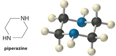
Piperazine is a diprotic base used to control intestinal parasites (“worms”) in pets and humans. A dog is given 500 mg (5.80 mmol) of piperazine (\(pK_{b1}\) = 4.27, \(pK_{b2}\) = 8.67). If the dog’s stomach initially contains 100 mL of 0.10 M HCl (pH = 1.00), calculate the pH of the stomach contents after ingestion of the piperazine.

Answer

pH=4.9

Summary

Plots of acid–base titrations generate titration curves that can be used to calculate the pH, the pOH, the \(pK_a\), and the \(pK_b\) of the system. To calculate pH at any point in a titration, the amounts of all species must first be determined using the stoichiometry of the neutralization reaction. Then, equilibrium methods can be used to determine the pH. In titrations of polyprotic acids or bases, the neutralization typically occurs in discrete steps that can be treated separately to calculate pH.