
27.2: The Chemical Bond in the Hydrogen Molecule
- Page ID
- 416119

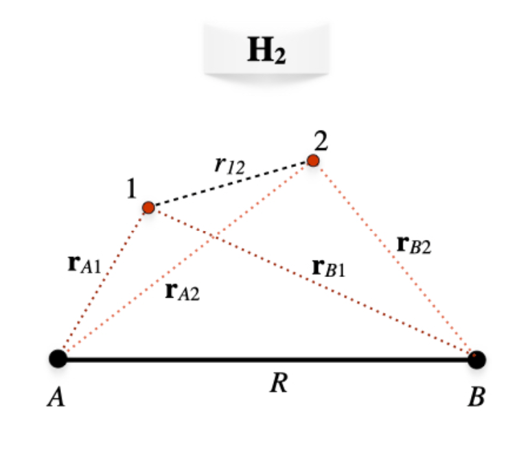
We can now examine the formation of the two-electron chemical bond in the \(\text{H}_2\) molecule. With reference to figure \(\PageIndex{1}\), the molecular Hamiltonian for \(\text{H}_2\) in a.u. in the Born-Oppenheimer approximation will be:
\[\begin{equation} \begin{aligned} \hat{H} &= \hat{H}_e+\dfrac{1}{R} \\ &=\left( -\dfrac{1}{2}\nabla^2_1-\dfrac{1}{\mathbf{r}_{A1}}-\dfrac{1}{\mathbf{r}_{B1}} \right)+\left( -\dfrac{1}{2}\nabla^2_2-\dfrac{1}{\mathbf{r}_{A2}}-\dfrac{1}{\mathbf{r}_{B2}} \right)+\dfrac{1}{r_{12}}+\dfrac{1}{R}\\ &= \hat{h}_1+\hat{h}_2+\dfrac{1}{r_{12}}+\dfrac{1}{R}, \end{aligned} \end{equation}\label{28.2.1} \]
where \(\hat{h}\) is the one-electron Hamiltonian. As for the previous case, we can build the first approximation to the molecular wave function by considering two \(1s\) atomic orbitals \(a(\mathbf{r}_1)\) and \(b(\mathbf{r}_2)\) centered at \(A\) and \(B\), respectively, having an overlap \(S\). If we Neglect the electron-electron repulsion term, \(\dfrac{1}{r_{12}}\), the resulting Hartree-Fock equations are exactly the same as in the previous case. The most important difference, though, is that in this case we need to consider the spin of the two electrons. Proceeding similarly to what we have done for the many-electron atom in chapter 26, we can build an antisymmetric wave function for \(\text{H}_2\) using a Slater determinant of doubly occupied MOs. For the ground state, we can use the lowest energy orbital obtained from the solution of the Hartree-Fock equations, which we already obtained in Equation 28.1.8. Using a notation that is based on the symmetry of the molecule, this bonding orbital in \(\text{H}_2\) is usually called \(\sigma_g\), where \(\sigma\) refers to the \(\sigma\) bond that forms between the two atoms. The Slater determinant for the ground state is therefore:\(^1\)
\[ \Psi (\mathbf{x}_{1},\mathbf{x}_{2})= |\sigma_{g}\phi_{\uparrow},\sigma_{g}\phi_{\downarrow}\rangle,=\sigma_{g}(\mathbf{r}_1)\sigma_{g}(\mathbf{r}_2) \dfrac{1}{\sqrt{2}} \left[ \phi_{\uparrow}\phi_{\downarrow} - \phi_{\downarrow}\phi_{\uparrow} \right], \label{28.2.2} \]
where:
\[ \sigma_{g}=\varphi_{+}=\dfrac{\left(\psi_{100}\right)_A+\left(\psi_{100}\right)_B}{\sqrt{2+2S}}. \label{28.2.3} \]
The energies and the resulting MO diagram is similar to that for \(\mathrm{H}_2^+\), with the only difference that two electron will be described by the same \(\sigma_g\) MO (figure \(\PageIndex{2}\)).
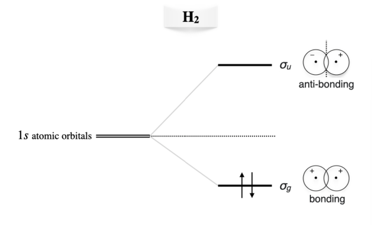 Figure \(\PageIndex{2}\): Molecular orbitals diagram for the hydrogen molecule.
As for the many-electron atoms, the Hartree-Fock method is just an approximation to the exact solution. The accurate theoretical value for the bond energy at the bond distance of \(R_e=1.4\;a_0\) is \(E= -0.17447\;E_h\). The variational result obtained with the wave function in Equation \ref{28.2.2} is \(E= -0.12778\;E_h\), which is \(\sim 73 \%\) of the exact value. The variational coefficient (i.e., the orbital exponent, \(c_0\), that enters the \(1s\) orbital formula \(\psi_{100}=\dfrac{1}{\pi}\exp[c_0r]\)) is optimized at \(c_0=1.1695\), a value that shows how the orbitals significantly contract due to spherical polarization.
If we scan the Born-Oppenheimer energy landscape using the wave function in Equation \ref{28.2.2} as we have done for \(\mathrm{H}_2^+\), we obtain the plot in figure \(\PageIndex{3}\).
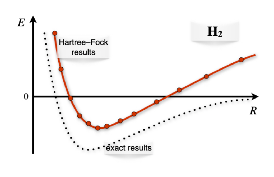
As we can see, the Hartree-Fock results for \(\mathrm{H}_2\) describes the formation of the bond qualitatively around the bond distance (minimum of the curve), but they fail to describe the molecule at dissociation. This happens because in Equation \ref{28.2.2} both electrons are in the same orbital with opposite spin (electrons are coupled), and the orbital is shared among both centers. At dissociation, this corresponds to an erroneous ionic dissociation state where both electron are localized on either one of the two centers (this center is therefore negatively charged), with the other proton left without electrons. This is in contrast with the correct dissociation, where each electron should be localized around each center (and therefore, it should be uncoupled from the other electron). This error is once again the result of the approximations that are necessary to treat the TISEq of a many-electron system. It is obviously not a failure of quantum mechanics, and it can be easily corrected using more accurate approximations on modern computers.
- Compare this equation to (10.6) for the helium atom.