27.1: The Chemical Bond in the Hydrogen Molecular Cation

This system has only one electron, but since its geometry is not spherical (figure \(\PageIndex{1}\)), the TISEq cannot be solved analytically as for the hydrogen atom.

Figure \(\PageIndex{1}\): Geometry of the hydrogen molecular cation.

The electron is at point \(P\), while the two protons are at position \(A\) and \(B\) at a fixed distance \(R\). Using the Born-Oppenheimer approximation we can write the one-electron molecular Hamiltonian in a.u. as:

\[ \hat{H} = \hat{H}_e+\dfrac{1}{R} = \left( -\dfrac{1}{2}\nabla^2-\dfrac{1}{\mathbf{r}_A}-\dfrac{1}{\mathbf{r}_B} \right)+\dfrac{1}{R} \label{28.1.1} \]

As a first approximation to the variational wave function, we can build the one-electron molecular orbital (MO) by linearly combine two \(1s\) hydrogenic orbitals centered at \(A\) and \(B\), respectively:

\[ \varphi = c_1 a + c_2 b, \label{28.1.2} \]

with:

\[ \begin{equation} \begin{aligned} a &= 1s_A = \left( \psi_{100} \right)_A\\ b &= 1s_B = \left( \psi_{100} \right)_B. \end{aligned} \end{equation}\label{28.1.3} \]

Using Equation 27.3.2 and considering that the nuclei are identical, we can define the integrals \(H_{aa}=H_{bb}, H_{ab}=H_{ba}\) and \(S_{ab}=S\) (while \(S_{aa}=1\) because the hydrogen atom orbitals are normalized). The secular equation, Equation 27.3.4 can then be written:

\[ \begin{vmatrix} H_{aa}-E & H_{ab}-ES \\\ H_{ab}-ES & H_{aa}-E \end{vmatrix}=0 \label{28.1.4} \]

The expansion of the determinant results into:

\[ \begin{equation} \begin{aligned} (H_{aa}-E)^2 &=(H_{ab}-ES)^2 \\ H_{aa}-E &= \pm (H_{ab}-ES), \\ \end{aligned} \end{equation}\label{28.1.5} \]

with roots:

\[ \begin{equation} \begin{aligned} E_{+} &= \dfrac{H_{aa}+H_{ab}}{1+S} = H_{aa}+\dfrac{H_{ba}-SH_{aa}}{1+S}, \\ E_{-} &= \dfrac{H_{aa}-H_{ab}}{1-S} = H_{aa}-\dfrac{H_{ba}-SH_{aa}}{1-S}, \end{aligned} \end{equation}\label{28.1.6} \]

the first corresponding to the ground state, the second to the first excited state. Solving for the best value for the coefficients of the linear combination for the ground state \(E_{+}\), we obtain:

\[ c_1=c_2=\dfrac{1}{\sqrt{2+2S}}, \label{28.1.7} \]

which gives the bonding MO:

\[ \varphi_{+}=\dfrac{a+b}{\sqrt{2+2S}}. \label{28.1.8} \]

Proceeding similarly for the excited state, we obtain:

\[ c_1=\dfrac{1}{\sqrt{2-2S}}\;\quad c_2=-\dfrac{1}{\sqrt{2-2S}}, \label{28.1.9} \]

which gives the antibonding MO:

\[ \varphi_{-}=\dfrac{b-a}{\sqrt{2-2S}}. \label{28.1.10} \]

These results can be summarized in the molecular orbital diagram of figure \(\PageIndex{2}\) We notice that the splitting of the doubly degenerate atomic level under the interaction is non-symmetric for \(S\neq0\), the antibonding level being more repulsive and the bonding less attractive than the symmetric case occurring for \(S = 0\).

Figure \(\PageIndex{2}\): Molecular orbitals diagram for the hydrogen molecular cation.

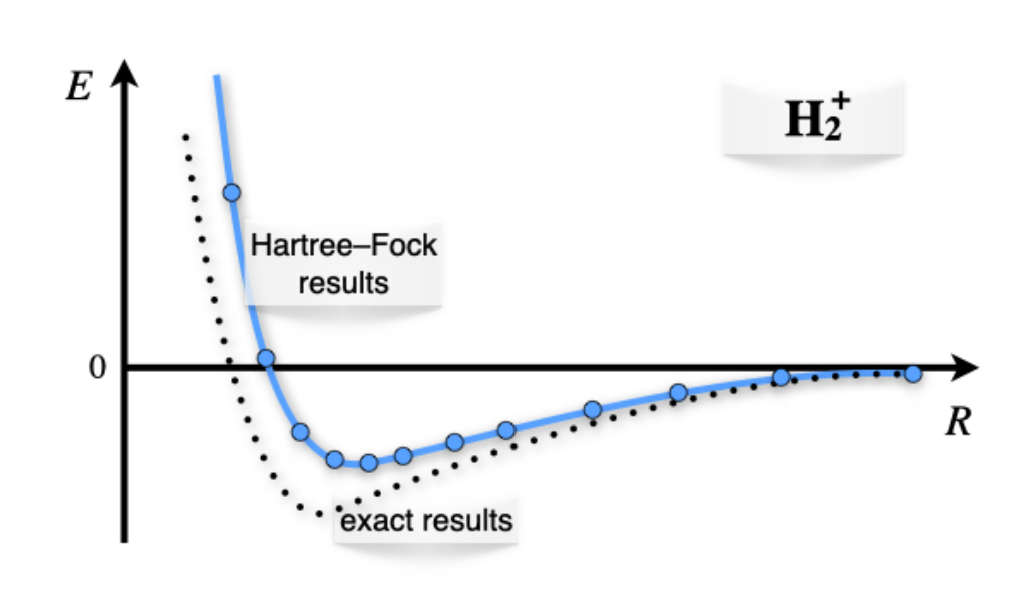
Calculating the values for the integrals and repeating these calculations for different internuclear distances, \(R\), results in the plot of figure \(\PageIndex{3}\) As we see from the plots, the ground state solution is negative for a vast portion of the plot. The energy is negative because the electronic energy calculated with the bonding orbital is lower than the nuclear repulsion. In other words, the creation of the molecular orbital stabilizes the molecular configuration versus the isolated fragments (one hydrogen atom and one proton).

Figure \(\PageIndex{3}\): Born-Oppenheimer energy landscape for the hydrogen molecular cation.