11.3: Critical Phenomena

Compressibility factors

The compressibility factor is a correction coefficient that describes the deviation of a real gas from ideal gas behaviour. It is usually represented with the symbol \(z\), and is calculated as:

\[ z=\dfrac{\overline{V}}{\overline{V}_{\text{ideal}}} = \dfrac{P \overline{V}}{RT}. \label{11.3.1} \]

It is evident from Equation \ref{11.3.1} that the compressibility factor is dependent on the pressure, and for an ideal gas \(z=1\) always. For a non-ideal gas at any given pressure, \(z\) can be higher or lower than one, separating the behavior of non-ideal gases into two possibilities. The dependence of the compressibility factor against pressure is represented for \(\mathrm{H}_2\) and \(\mathrm{CO}_2\) in Figure \(\PageIndex{5}\).

Figure \(\PageIndex{1}\): Non-Ideal Gases Behaviors.

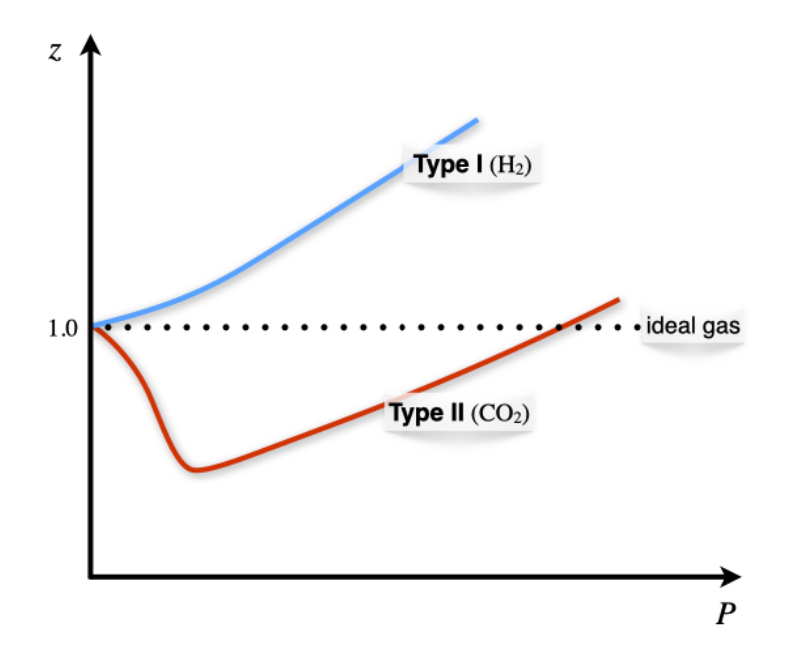
The two types of possible behaviors are differentiated based on the compressibility factor at \(P\rightarrow 0\). To analyze these situations we can use the vdW equation to calculate the compressibility factor as:

\[ z= \dfrac{\overline{V}}{RT} \left( \dfrac{RT}{\overline{V}-b} -\dfrac{a}{\overline{V}^2} \right). \label{11.3.2} \]

and then we can differentiate this equation at constant temperature with respect to changes in the pressure near \(P=0\), to obtain:

\[ \left. \left( \dfrac{\partial z}{\partial P}\right)_T \right|_{P=0} = \dfrac{1}{RT} \left( b -\dfrac{a}{RT} \right). \label{11.3.3} \]

which is then interpreted as follows:

• Type I gases: \(b>\dfrac{a}{RT} \; \Rightarrow \; \dfrac{\partial z}{\partial P} > 0\) molecular size dominates (\(\mathrm{H}_2-\)like behavior).
• Type II gases: \(b<\dfrac{a}{RT} \; \Rightarrow \; \dfrac{\partial z}{\partial P} < 0\) attractive forces dominates (\(\mathrm{CO}_2-\)like behavior).

The dependence of the compressibility factor as a function of temperature (Figure \(\PageIndex{6}\)) results in different plots for each of the two types of behavior.

Figure \(\PageIndex{2}\): Temperature Dependence of the Compressibility Factor.

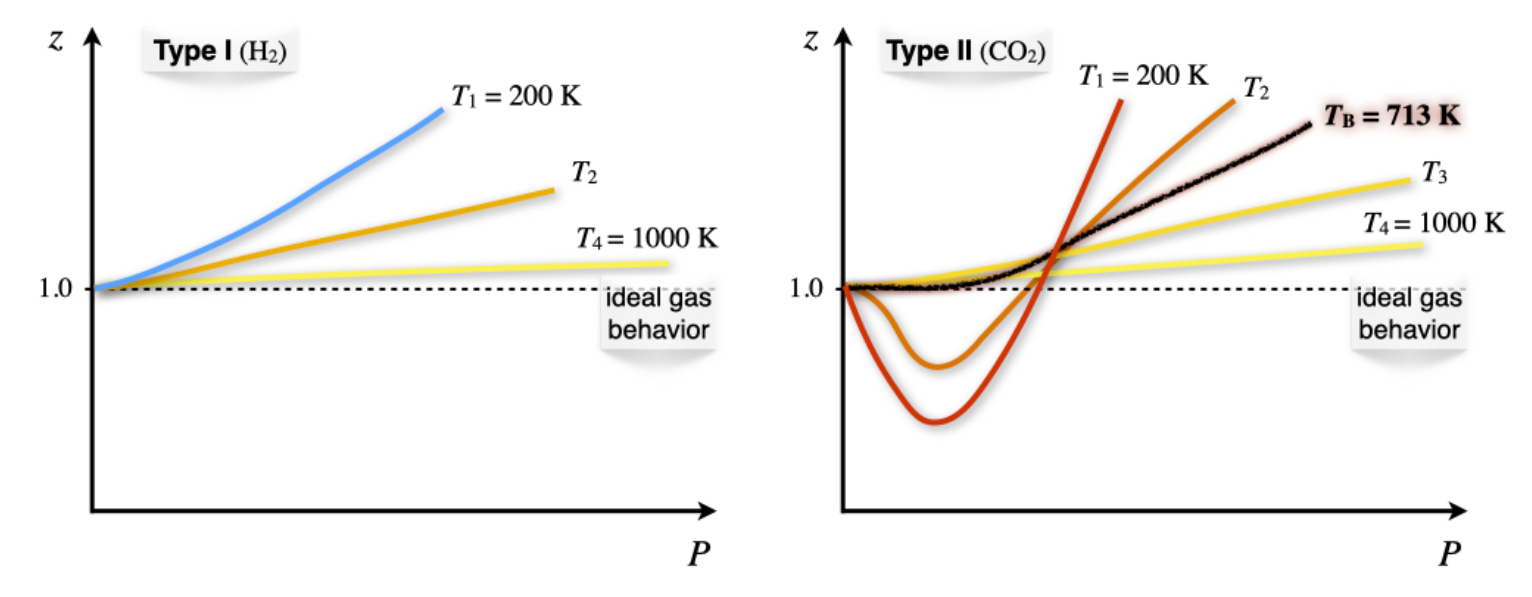
Both type I and type II non-ideal gases will approach the ideal gas behavior as \(T\rightarrow \infty\), because \(\dfrac{1}{RT}\rightarrow 0\) as \(T\rightarrow \infty\). For type II gases, there are three interesting situations:

• At low \(T\): \(b<\dfrac{a}{RT} \; \Rightarrow \; \dfrac{\partial z}{\partial P} < 0,\) which is the behavior described above.
• At high \(T\): \(b>\dfrac{a}{RT} \; \Rightarrow \; \dfrac{\partial z}{\partial P} > 0,\) which is the same behavior of type I gases.
• At a very specific temperature, inversion will occur (i.e., at \(T=713 \; \mathrm{K}\) for \(\mathrm{CO}_2\)). This temperature is called the Boyle temperature, \(T_{\mathrm{B}}\), and is the temperature at which the attractive and repulsive forces balance out. It can be calculated from the vdW equation, since \(b-\dfrac{a}{RT_{\mathrm{B}}}=0 \; \Rightarrow \; T_{\mathrm{B}}=\dfrac{a}{bR}.\) At the Boyle’s temperature a type II gas shows ideal gas behavior over a large range of pressure.

Phase diagram of a non-ideal gas

Let’s now turn our attention to the \(PV\) phase diagram of a non-ideal gas, reported in Figure \(\PageIndex{7}\).

Figure \(\PageIndex{3}\): The Pressure–Volume Diagram of a Non-Ideal Gas.

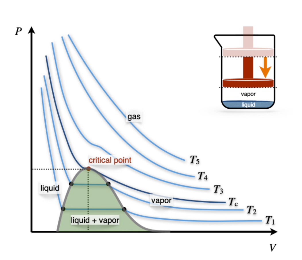
We can start the analysis from an isotherm at a high temperature. Since every gas will behave as an ideal gas at those conditions, the corresponding isotherms will look similar to those of an ideal gas (\(T_5\) and \(T_4\) in Figure \(\PageIndex{3}\)). Lowering the temperature, we start to see the deviation from ideality getting more prominent (\(T_3\) in Figure \(\PageIndex{3}\)) until we reach a particular temperature called the critical temperature, \(T_c\).

Definition: Critical Temperature

The temperature above which no appearance of a second phase is observed, regardless of how high the pressure becomes.

At the critical temperature and below, the gas liquefies when the pressure is increased. For this reason, the liquefaction of a gas is called a critical phenomenon.

The critical temperature is the coordinate of a unique point, called the critical point, that can be visualized in the three-dimensional \(T,P,V\) diagram of each gas (Figure \(\PageIndex{4}\))\(^1\).

Figure \(\PageIndex{4}\): The three-dimensional diagram. (CC By-SA 3.0 unported; Donald L. Smith via Wikipedia)

The critical point has coordinates \({T_c,P_c, \overline{V}_c}\). These critical coordinates can be determined from the vdW equation at \(T_c\), as:

\[ T_c=\dfrac{8a}{27Rb} \qquad P_c=\dfrac{a}{27b^2} \qquad \overline{V}_c=3b, \label{11.3.4} \]

These relations are used, in practice, to determine the vdW constants \(a,b\) from the experimentally measured critical isotherms.

The critical compressibility factor, \(z_c\), is predicted from the vdW equation at:

\[ z_c=\dfrac{P_c \overline{V}_c}{R T_c}=\left( \dfrac{a}{27b^2} \right) \left( \dfrac{3b}{R} \right) \left( \dfrac{27Rb}{8a} \right) = \dfrac{3}{8} = 0.375, \label{11.3.5} \]

a value that is independent of the gas. Experimentally measured values of \(z_c\) for different non-ideal gases are in the range of 0.2–0.3. These values can be used to infer the accuracy of the vdW equation for each non-ideal gas. Since the experimental \(z_c\) is usually lower than the one calculated from the vdW equation, we can deduce that the vdW equation overestimates the critical molar volume.

Notice how slicing the \(PT\overline{V}\) diagram at constant \(T\) results in the \(PV\) diagram that we reported in Figure \(\PageIndex{4}\). On the other hand, slicing the \(PT\overline{V}\) diagram at constant \(P\) results in the \(PT\) diagram that we will examine in detail in the next chapter.