5.6: Temperature-Programmed Techniques
- Page ID
- 25386
\( \newcommand{\vecs}[1]{\overset { \scriptstyle \rightharpoonup} {\mathbf{#1}} } \)
\( \newcommand{\vecd}[1]{\overset{-\!-\!\rightharpoonup}{\vphantom{a}\smash {#1}}} \)
\( \newcommand{\dsum}{\displaystyle\sum\limits} \)
\( \newcommand{\dint}{\displaystyle\int\limits} \)
\( \newcommand{\dlim}{\displaystyle\lim\limits} \)
\( \newcommand{\id}{\mathrm{id}}\) \( \newcommand{\Span}{\mathrm{span}}\)
( \newcommand{\kernel}{\mathrm{null}\,}\) \( \newcommand{\range}{\mathrm{range}\,}\)
\( \newcommand{\RealPart}{\mathrm{Re}}\) \( \newcommand{\ImaginaryPart}{\mathrm{Im}}\)
\( \newcommand{\Argument}{\mathrm{Arg}}\) \( \newcommand{\norm}[1]{\| #1 \|}\)
\( \newcommand{\inner}[2]{\langle #1, #2 \rangle}\)
\( \newcommand{\Span}{\mathrm{span}}\)
\( \newcommand{\id}{\mathrm{id}}\)
\( \newcommand{\Span}{\mathrm{span}}\)
\( \newcommand{\kernel}{\mathrm{null}\,}\)
\( \newcommand{\range}{\mathrm{range}\,}\)
\( \newcommand{\RealPart}{\mathrm{Re}}\)
\( \newcommand{\ImaginaryPart}{\mathrm{Im}}\)
\( \newcommand{\Argument}{\mathrm{Arg}}\)
\( \newcommand{\norm}[1]{\| #1 \|}\)
\( \newcommand{\inner}[2]{\langle #1, #2 \rangle}\)
\( \newcommand{\Span}{\mathrm{span}}\) \( \newcommand{\AA}{\unicode[.8,0]{x212B}}\)
\( \newcommand{\vectorA}[1]{\vec{#1}} % arrow\)
\( \newcommand{\vectorAt}[1]{\vec{\text{#1}}} % arrow\)
\( \newcommand{\vectorB}[1]{\overset { \scriptstyle \rightharpoonup} {\mathbf{#1}} } \)
\( \newcommand{\vectorC}[1]{\textbf{#1}} \)
\( \newcommand{\vectorD}[1]{\overrightarrow{#1}} \)
\( \newcommand{\vectorDt}[1]{\overrightarrow{\text{#1}}} \)
\( \newcommand{\vectE}[1]{\overset{-\!-\!\rightharpoonup}{\vphantom{a}\smash{\mathbf {#1}}}} \)
\( \newcommand{\vecs}[1]{\overset { \scriptstyle \rightharpoonup} {\mathbf{#1}} } \)
\(\newcommand{\longvect}{\overrightarrow}\)
\( \newcommand{\vecd}[1]{\overset{-\!-\!\rightharpoonup}{\vphantom{a}\smash {#1}}} \)
\(\newcommand{\avec}{\mathbf a}\) \(\newcommand{\bvec}{\mathbf b}\) \(\newcommand{\cvec}{\mathbf c}\) \(\newcommand{\dvec}{\mathbf d}\) \(\newcommand{\dtil}{\widetilde{\mathbf d}}\) \(\newcommand{\evec}{\mathbf e}\) \(\newcommand{\fvec}{\mathbf f}\) \(\newcommand{\nvec}{\mathbf n}\) \(\newcommand{\pvec}{\mathbf p}\) \(\newcommand{\qvec}{\mathbf q}\) \(\newcommand{\svec}{\mathbf s}\) \(\newcommand{\tvec}{\mathbf t}\) \(\newcommand{\uvec}{\mathbf u}\) \(\newcommand{\vvec}{\mathbf v}\) \(\newcommand{\wvec}{\mathbf w}\) \(\newcommand{\xvec}{\mathbf x}\) \(\newcommand{\yvec}{\mathbf y}\) \(\newcommand{\zvec}{\mathbf z}\) \(\newcommand{\rvec}{\mathbf r}\) \(\newcommand{\mvec}{\mathbf m}\) \(\newcommand{\zerovec}{\mathbf 0}\) \(\newcommand{\onevec}{\mathbf 1}\) \(\newcommand{\real}{\mathbb R}\) \(\newcommand{\twovec}[2]{\left[\begin{array}{r}#1 \\ #2 \end{array}\right]}\) \(\newcommand{\ctwovec}[2]{\left[\begin{array}{c}#1 \\ #2 \end{array}\right]}\) \(\newcommand{\threevec}[3]{\left[\begin{array}{r}#1 \\ #2 \\ #3 \end{array}\right]}\) \(\newcommand{\cthreevec}[3]{\left[\begin{array}{c}#1 \\ #2 \\ #3 \end{array}\right]}\) \(\newcommand{\fourvec}[4]{\left[\begin{array}{r}#1 \\ #2 \\ #3 \\ #4 \end{array}\right]}\) \(\newcommand{\cfourvec}[4]{\left[\begin{array}{c}#1 \\ #2 \\ #3 \\ #4 \end{array}\right]}\) \(\newcommand{\fivevec}[5]{\left[\begin{array}{r}#1 \\ #2 \\ #3 \\ #4 \\ #5 \\ \end{array}\right]}\) \(\newcommand{\cfivevec}[5]{\left[\begin{array}{c}#1 \\ #2 \\ #3 \\ #4 \\ #5 \\ \end{array}\right]}\) \(\newcommand{\mattwo}[4]{\left[\begin{array}{rr}#1 \amp #2 \\ #3 \amp #4 \\ \end{array}\right]}\) \(\newcommand{\laspan}[1]{\text{Span}\{#1\}}\) \(\newcommand{\bcal}{\cal B}\) \(\newcommand{\ccal}{\cal C}\) \(\newcommand{\scal}{\cal S}\) \(\newcommand{\wcal}{\cal W}\) \(\newcommand{\ecal}{\cal E}\) \(\newcommand{\coords}[2]{\left\{#1\right\}_{#2}}\) \(\newcommand{\gray}[1]{\color{gray}{#1}}\) \(\newcommand{\lgray}[1]{\color{lightgray}{#1}}\) \(\newcommand{\rank}{\operatorname{rank}}\) \(\newcommand{\row}{\text{Row}}\) \(\newcommand{\col}{\text{Col}}\) \(\renewcommand{\row}{\text{Row}}\) \(\newcommand{\nul}{\text{Nul}}\) \(\newcommand{\var}{\text{Var}}\) \(\newcommand{\corr}{\text{corr}}\) \(\newcommand{\len}[1]{\left|#1\right|}\) \(\newcommand{\bbar}{\overline{\bvec}}\) \(\newcommand{\bhat}{\widehat{\bvec}}\) \(\newcommand{\bperp}{\bvec^\perp}\) \(\newcommand{\xhat}{\widehat{\xvec}}\) \(\newcommand{\vhat}{\widehat{\vvec}}\) \(\newcommand{\uhat}{\widehat{\uvec}}\) \(\newcommand{\what}{\widehat{\wvec}}\) \(\newcommand{\Sighat}{\widehat{\Sigma}}\) \(\newcommand{\lt}{<}\) \(\newcommand{\gt}{>}\) \(\newcommand{\amp}{&}\) \(\definecolor{fillinmathshade}{gray}{0.9}\)There are a range of techniques for studying surface reactions and molecular adsorption on surfaces which utilize temperature-programming to discriminate between processes with different activation parameters. Of these, the most useful for single crystal studies is: Temperature Programmed Desorption (TPD). When the technique is applied to a system in which the adsorption process is, at least in part, irreversible and T-programming leads to surface reactions, then this technique is often known as: Temperature Programmed Reaction Spectroscopy (TPRS)
However, there is no substantive difference between TPRS and TPD. The basic experiment is very simple, involving
- Adsorption of one or more molecular species onto the sample surface at low temperature (frequently 300 K, but sometimes sub-ambient).
- Heating of the sample in a controlled manner (preferably so as to give a linear temperature ramp) whilst monitoring the evolution of species from the surface back into the gas phase.
In modern implementations of the technique the detector of choice is a small, quadrupole mass spectrometer (QMS) and the whole process is carried out under computer control with quasi-simultaneous monitoring of a large number of possible products.
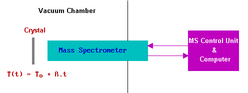
The data obtained from such an experiment consists of the intensity variation of each recorded mass fragment as a function of time / temperature. In the case of a simple reversible adsorption process it may only be necessary to record one signal - that attributable to the molecular ion of the adsorbate concerned.
The graph below shows data from a TPD experiment following adsorption of CO onto a Pd(111) crystal at 300 K.
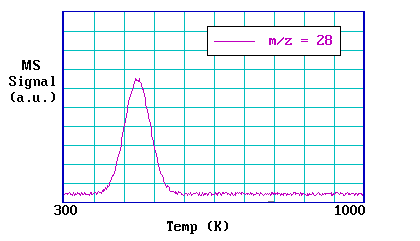
Since mass spectrometric detection is used the sensitivity of the technique is good with attainable detection limits below 0.1% of a monolayer of adsorbate.
The following points are worth noting:
- The area under a peak is proportional to the amount originally adsorbed, i.e. proportional to the surface coverage.
- The kinetics of desorption (obtained from the peak profile and the coverage dependence of the desorption characteristics) give information on the state of aggregation of the adsorbed species e.g. molecular v's dissociative.
- The position of the peak (the peak temperature) is related to the enthalpy of adsorption, i.e. to the strength of binding to the surface.
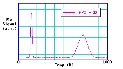
One implication of the last point, is that if there is more than one binding state for a molecule on a surface (and these have significantly different adsorption enthalpies) then this will give rise to multiple peaks in the TPD spectrum.
The graph below shows data from a TPD experiment following adsorption of oxygen on Pt(111) at 80 K.
Theory of TPD
As discussed in Section 2.6, the rate of desorption of a surface species will in general be given by an expression of the form:
\[R_{des} = ν N^x \exp \left( \dfrac{- E_a^{des} }{ R T} \right) \label{1}\]
with
- \(R_{des}\) - desorption rate ( \(= -dN/dt\) )
- \(x\) - kinetic order of desorption (typically 0,1 or 2)
- \(E_a^{des}\) - activation energy for desorption
In a temperature programmed desorption experiment in which the temperature is increased linearly with time from some initial temperature \(T_o\), then:
\[T = T_o + βt \label{2a}\]
and
\[dT = β\,dt \label{2b}\]
The intensity of the desorption signal, I(T), is proportional to the rate at which the surface concentration of adsorbed species is decreasing. This is obtained by combining [1] and [2] to give
\[ I(T) \propto \dfrac{dN}{dT} = \dfrac{\nu N^x}{\beta} e^{-E_a^{des}/RT} \label{3}\]
This problem may also be considered in a rather simplistic graphical way -the key to this is to recognize that the expression for the desorption signal given in the above equation is basically a product of a coverage term ( \(N^x\) - where \(N\) depends on \(T\) ) and an exponential term (involving both \(E_a\) and \(T\) ).
Initially, at low temperatures \(E_a >> RT\) and the exponential term is vanishing small. However, as the temperature is increased this term begins to increase very rapidly when the value of RT approaches that of the activation energy, \(E_a\).
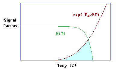
By contrast, the pre-exponential term is dependent upon the coverage, N(T), at the temperature concerned - this term will remain at the initial value until the desorption rate becomes of significance as a result of the increasing exponential term. Thereafter, it will decrease ever more rapidly until the coverage is reduced to zero. The shaded area is an approximate representation of the product of these two functions, and hence also an approximate representation for the desorption signal itself - whilst this illustration may be overly simplistic it does clearly show why the desorption process gives rise to a well-defined desorption peak.
If you wish to see exactly how the various factors such as the kinetic order and initial coverage influence the desorption profile then try out the Interactive Demonstration of Temperature Programmed Desorption (note - this is based on the formulae given in Section 2.6 ); we will however continue to look at one particular case in a little more detail.
CASE I (Molecular adsorption)
In this case the desorption kinetics will usually be first order (i.e. \(x = 1\) ). The maximum desorption signal in the \(I(T)\) trace will occur when ( \(dI / dT\) ) = 0, i.e. when
\[ \dfrac{d}{dT}\left[ \dfrac{\nu N}{\beta} \; \exp \left( \dfrac{-E_a^{des}}{RT} \right) \right] = 0 \]
Hence, remembering that the surface coverage changes with temperature i.e., \(N = N(T)\),

where we have substituted \(E_a\) for \(E_a^{des}\) purely for clarity of presentation. Substituting for \(dN/dT\) from eq. 3 then gives

The solution is given by setting the expression in square brackets to be equal to zero, i.e.,
\[ \dfrac{E_a}{RT^2_p}=\dfrac{\nu}{\beta}\; \exp \left(\dfrac{-E_a}{RT_p} \right)\]
where we have now defined the temperature at which the desorption maximum occurs to be T = Tp (the peak temperature ).
Unfortunately, this equation cannot be re-arranged to make \(T_p\) the subject (i.e. to give a simple expression of the form Tp = .....), but we can note that:
- as \(E_a^{des}\) (the activation energy for desorption) increases, then so \(T_p\) (the peak temperature) increases.
- the peak temperature is not dependent upon, and consequently does not change with, the initial coverage, \(N_t=0\).
- the shape of the desorption peak will tend to be asymmetric, with the signal decreasing rapidly after the desorption maximum.
Temperature Programmed Reaction Spectroscopy
In TPRS a number of desorption products will normally be detected in any one experiment - this is where mass spectrometric detection and multiple ion monitoring really becomes essential. A good example of TPRS results are those obtained from dosing formic acid (HCOOH) onto a copper surface.
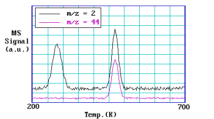
The spectra contain two regions of interest - the first at around room temperature where there is desorption of hydrogen \(H_2\) with \(m/z = 2\) alone, and the second between 400 K and 500 K, where there are coincident desorption peaks attributable to hydrogen and carbon dioxide \(CO_2\) with \(m/z = 44\).
The lower temperature hydrogen peak is at about the same temperature at which hydrogen atoms recombine and desorb as molecular hydrogen from a hydrogen-dosed Cu(110) surface i.e. the kinetics of its evolution into the gas phase are those of the normal recombinative desorption process. By contrast, the higher temperature hydrogen peak is observed well above the normal hydrogen desorption temperature - its appearance must be governed by the kinetics of decomposition of another surface species. The carbon dioxide peak must also be decomposition limited since on clean Cu(110) carbon dioxide itself is only weakly physisorbed at very low temperatures.
More generally, coincident desorption of two species at temperatures well above their normal desorption temperatures is characteristic of the decomposition of a more complex surface species.


