Entropy of Mixing
- Page ID
- 1945
\( \newcommand{\vecs}[1]{\overset { \scriptstyle \rightharpoonup} {\mathbf{#1}} } \)
\( \newcommand{\vecd}[1]{\overset{-\!-\!\rightharpoonup}{\vphantom{a}\smash {#1}}} \)
\( \newcommand{\dsum}{\displaystyle\sum\limits} \)
\( \newcommand{\dint}{\displaystyle\int\limits} \)
\( \newcommand{\dlim}{\displaystyle\lim\limits} \)
\( \newcommand{\id}{\mathrm{id}}\) \( \newcommand{\Span}{\mathrm{span}}\)
( \newcommand{\kernel}{\mathrm{null}\,}\) \( \newcommand{\range}{\mathrm{range}\,}\)
\( \newcommand{\RealPart}{\mathrm{Re}}\) \( \newcommand{\ImaginaryPart}{\mathrm{Im}}\)
\( \newcommand{\Argument}{\mathrm{Arg}}\) \( \newcommand{\norm}[1]{\| #1 \|}\)
\( \newcommand{\inner}[2]{\langle #1, #2 \rangle}\)
\( \newcommand{\Span}{\mathrm{span}}\)
\( \newcommand{\id}{\mathrm{id}}\)
\( \newcommand{\Span}{\mathrm{span}}\)
\( \newcommand{\kernel}{\mathrm{null}\,}\)
\( \newcommand{\range}{\mathrm{range}\,}\)
\( \newcommand{\RealPart}{\mathrm{Re}}\)
\( \newcommand{\ImaginaryPart}{\mathrm{Im}}\)
\( \newcommand{\Argument}{\mathrm{Arg}}\)
\( \newcommand{\norm}[1]{\| #1 \|}\)
\( \newcommand{\inner}[2]{\langle #1, #2 \rangle}\)
\( \newcommand{\Span}{\mathrm{span}}\) \( \newcommand{\AA}{\unicode[.8,0]{x212B}}\)
\( \newcommand{\vectorA}[1]{\vec{#1}} % arrow\)
\( \newcommand{\vectorAt}[1]{\vec{\text{#1}}} % arrow\)
\( \newcommand{\vectorB}[1]{\overset { \scriptstyle \rightharpoonup} {\mathbf{#1}} } \)
\( \newcommand{\vectorC}[1]{\textbf{#1}} \)
\( \newcommand{\vectorD}[1]{\overrightarrow{#1}} \)
\( \newcommand{\vectorDt}[1]{\overrightarrow{\text{#1}}} \)
\( \newcommand{\vectE}[1]{\overset{-\!-\!\rightharpoonup}{\vphantom{a}\smash{\mathbf {#1}}}} \)
\( \newcommand{\vecs}[1]{\overset { \scriptstyle \rightharpoonup} {\mathbf{#1}} } \)
\(\newcommand{\longvect}{\overrightarrow}\)
\( \newcommand{\vecd}[1]{\overset{-\!-\!\rightharpoonup}{\vphantom{a}\smash {#1}}} \)
\(\newcommand{\avec}{\mathbf a}\) \(\newcommand{\bvec}{\mathbf b}\) \(\newcommand{\cvec}{\mathbf c}\) \(\newcommand{\dvec}{\mathbf d}\) \(\newcommand{\dtil}{\widetilde{\mathbf d}}\) \(\newcommand{\evec}{\mathbf e}\) \(\newcommand{\fvec}{\mathbf f}\) \(\newcommand{\nvec}{\mathbf n}\) \(\newcommand{\pvec}{\mathbf p}\) \(\newcommand{\qvec}{\mathbf q}\) \(\newcommand{\svec}{\mathbf s}\) \(\newcommand{\tvec}{\mathbf t}\) \(\newcommand{\uvec}{\mathbf u}\) \(\newcommand{\vvec}{\mathbf v}\) \(\newcommand{\wvec}{\mathbf w}\) \(\newcommand{\xvec}{\mathbf x}\) \(\newcommand{\yvec}{\mathbf y}\) \(\newcommand{\zvec}{\mathbf z}\) \(\newcommand{\rvec}{\mathbf r}\) \(\newcommand{\mvec}{\mathbf m}\) \(\newcommand{\zerovec}{\mathbf 0}\) \(\newcommand{\onevec}{\mathbf 1}\) \(\newcommand{\real}{\mathbb R}\) \(\newcommand{\twovec}[2]{\left[\begin{array}{r}#1 \\ #2 \end{array}\right]}\) \(\newcommand{\ctwovec}[2]{\left[\begin{array}{c}#1 \\ #2 \end{array}\right]}\) \(\newcommand{\threevec}[3]{\left[\begin{array}{r}#1 \\ #2 \\ #3 \end{array}\right]}\) \(\newcommand{\cthreevec}[3]{\left[\begin{array}{c}#1 \\ #2 \\ #3 \end{array}\right]}\) \(\newcommand{\fourvec}[4]{\left[\begin{array}{r}#1 \\ #2 \\ #3 \\ #4 \end{array}\right]}\) \(\newcommand{\cfourvec}[4]{\left[\begin{array}{c}#1 \\ #2 \\ #3 \\ #4 \end{array}\right]}\) \(\newcommand{\fivevec}[5]{\left[\begin{array}{r}#1 \\ #2 \\ #3 \\ #4 \\ #5 \\ \end{array}\right]}\) \(\newcommand{\cfivevec}[5]{\left[\begin{array}{c}#1 \\ #2 \\ #3 \\ #4 \\ #5 \\ \end{array}\right]}\) \(\newcommand{\mattwo}[4]{\left[\begin{array}{rr}#1 \amp #2 \\ #3 \amp #4 \\ \end{array}\right]}\) \(\newcommand{\laspan}[1]{\text{Span}\{#1\}}\) \(\newcommand{\bcal}{\cal B}\) \(\newcommand{\ccal}{\cal C}\) \(\newcommand{\scal}{\cal S}\) \(\newcommand{\wcal}{\cal W}\) \(\newcommand{\ecal}{\cal E}\) \(\newcommand{\coords}[2]{\left\{#1\right\}_{#2}}\) \(\newcommand{\gray}[1]{\color{gray}{#1}}\) \(\newcommand{\lgray}[1]{\color{lightgray}{#1}}\) \(\newcommand{\rank}{\operatorname{rank}}\) \(\newcommand{\row}{\text{Row}}\) \(\newcommand{\col}{\text{Col}}\) \(\renewcommand{\row}{\text{Row}}\) \(\newcommand{\nul}{\text{Nul}}\) \(\newcommand{\var}{\text{Var}}\) \(\newcommand{\corr}{\text{corr}}\) \(\newcommand{\len}[1]{\left|#1\right|}\) \(\newcommand{\bbar}{\overline{\bvec}}\) \(\newcommand{\bhat}{\widehat{\bvec}}\) \(\newcommand{\bperp}{\bvec^\perp}\) \(\newcommand{\xhat}{\widehat{\xvec}}\) \(\newcommand{\vhat}{\widehat{\vvec}}\) \(\newcommand{\uhat}{\widehat{\uvec}}\) \(\newcommand{\what}{\widehat{\wvec}}\) \(\newcommand{\Sighat}{\widehat{\Sigma}}\) \(\newcommand{\lt}{<}\) \(\newcommand{\gt}{>}\) \(\newcommand{\amp}{&}\) \(\definecolor{fillinmathshade}{gray}{0.9}\)A gas will always flow into a newly available volume and does so because its molecules are rapidly bouncing off one another and hitting the walls of their container, readily moving into a new allowable space. It follows from the second law of thermodynamics that a process will occur in the direction towards a more probable state. In terms of entropy, this can be expressed as a system going from a state of lesser probability (less microstates) towards a state of higher probability (more microstates). This corresponds to increasing the \(W\) in the equation \( S=k_B\ln W \).
The Mixing of Ideal Gases
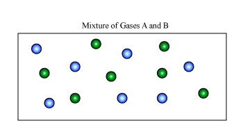
For our example, we shall again consider a simple system of two ideal gases, A and B, with a number of moles \( n_A \) and \( n_B \), at a certain constant temperature and pressure in volumes of \( V_A \) and \( V_B \), as shown in Figure \(\PageIndex{1A}\). These two gases are separated by a partition so they are each sequestered in their respective volumes. If we now remove the partition (like opening a window in the example above), we expect the two gases to randomly diffuse and form a homogenous mixture as we see in Figure \(\PageIndex{1B}\).

To calculate the entropy change, let us treat this mixing as two separate gas expansions, one for gas A and another for B. From the statistical definition of entropy, we know that
\[ \Delta S=nR\ln \dfrac{V_2}{V_1} \;. \nonumber \]
Now, for each gas, the volume \( V_1 \) is the initial volume of the gas, and \( V_2 \) is the final volume, which is both the gases combined, \( V_A+V_B \). So for the two separate gas expansions,
\[ \Delta S_A=n_A R\ln \dfrac{V_A+V_B}{V_A} \nonumber \]
\[ \Delta S_B=n_B R\ln \dfrac{V_A+V_B}{V_B} \nonumber \]
So to find the total entropy change for both these processes, because they are happening at the same time, we simply add the two changes in entropy together.
\[ \Delta_{mix}S = \Delta S_{A}+\Delta S_{B}=n_{A}R\ln \dfrac{V_{A}+V_{B}}{V_{A}}+n_{B}R\ln \dfrac{V_{A}+V_{B}}{V_{B}} \nonumber \]
Recalling the ideal gas law, PV=nRT, we see that the volume is directly proportional to the number of moles (Avogadro's Law), and since we know the number of moles we can substitute this for the volume:
\[ \Delta_{mix}S=n_{A}R\ln \dfrac{n_{A}+n_{B}}{n_{A}}+n_{B}R\ln \dfrac{n_{A}+n_{B}}{n_{B}} \nonumber \]
Now we recognize that the inverse of the term \( \frac{n_{A}+n_{B}}{n_{A}} \) is the mole fraction \( \chi_{A}=\frac{n_{A}}{n_{A}+n_{B}} \), and taking the inverse of these two terms in the above equation, we have:
\[ \Delta_{mix}S=-n_{A}R\ln \dfrac{n_A}{n_A+n_B}-n_BR\ln \dfrac{n_A}{n_A+n_B}\chi_{B} = -n_A R\ln \chi_A -n_B R\ln \chi_B \nonumber \]
since \(\ln x^{-1}=-\ln x\) from the rules for logarithms. If we now factor out R from each term:
\[ \Delta_{mix}S=-R(n_{A}\ln \chi_{A}+n_{B}\ln \chi_{B}) \nonumber \]
represents the equation for the entropy change of mixing. This equation is also commonly written with the total number of moles:
\[ \Delta_{mix}S=-nR(\chi_A \ln \chi_A+\chi_B\ln \chi_B) \label{Final} \]
where the total number of moles is \( n=n_A+n_B \)
Notice that when the two gases will be mixed, their mole fraction will be less than one, making the term inside the parentheses negative, and thus the entropy of mixing will always be positive. This observation makes sense, because as you add a component to another for a two-component solution, the mole fraction of the other component will decrease, and the log of a number less than 1 is negative. Multiplied by the negative in the front of the equation gives a positive quantity. Equation \(\ref{Final}\) applies to both ideal solutions and ideal gases.
References
- Chang, Raymond. Physical Chemistry for the Biosciences. Sausalito, California: University Science Books, 2005.
Outside Links
- Sattar, Simeen. "Thermodynamics of Mixing Real Gases." J. Chem. Educ. 2000 77 1361.

