8.61: Simulating Quantum Correlations with a Quantum Computer

According to Richard Feynman it takes a quantum computer to simulate quantum phenomena. In this tutorial we begin with a traditional quantum analysis of a well-know thought experiment involving correlated spin-1/2 particles. After that the operation of a quantum circuit designed to simulate the thought experiment is analyzed. It will be shown that the quantum analysis and the simulation lead to the same result for the expectation value for the experiment.

The Thought Experiment

A spin-1/2 pair is prepared in an entangled singlet state and the individual particles travel in opposite directions on the y-axis to a pair of Stern-Gerlach (SG) detectors which are set up to measure spin in the x-z plane.

\[ | \Psi_m \rangle = \frac{1}{ \sqrt{2}} \left[ | \uparrow_1 \rangle | \downarrow_2 \rangle - | \downarrow_1 \rangle | \uparrow_2 \rangle \right] = \frac{1}{ \sqrt{2}} \left[ \right] = \frac{1}{ \sqrt{2}} \begin{pmatrix} 0 \\ 1 \\ -1 \\ 0 \end{pmatrix} \nonumber \]

Particle A's spin is measured along with z-axis, and particle B's spin is measured at any angle θ with respect to the z-axis in the x-z plane. The experimental apparatus is shown below.

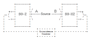
The single particle spin operator in the x-z plane is constructed from the Pauli spin operators in the x- and z-directions. θ is the angle of orientation of the measurement magnet with the z-axis.

\[ \begin{matrix} \sigma_z = \begin{pmatrix} 1 & 0 \\ 0 & -1 \end{pmatrix} & \sigma_x = \begin{pmatrix} 0 & 1 \\ 1 & 0 \end{pmatrix} & S( \theta) = \cos ( \theta) \sigma_z + \sin ( \theta) \sigma_x \rightarrow \begin{pmatrix} \cos \theta & \sin \theta \\ \sin \theta & - \cos \theta \end{pmatrix} \end{matrix} \nonumber \]

Tensor multiplication of S_A(0) and S_B(θ) creates a joint measurement operator for spins A and B.

\[ S_A (0) \otimes S_B ( \theta) = \begin{pmatrix} 1 & 0 \\ 0 & -1 \end{pmatrix} \otimes \begin{pmatrix} \cos \theta & \sin \theta \\ \sin \theta & - \cos \theta \end{pmatrix} = \begin{pmatrix} \cos \theta & \sin \theta & 0 & 0 \\ \sin \theta & - \cos \theta & 0 & 0 \\ 0 & 0 & - \cos \theta & - \sin \theta \\ 0 & 0 & - \sin \theta & \cos \theta \end{pmatrix} \nonumber \]

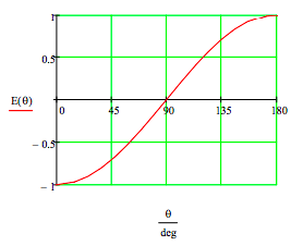
The expectation value as a function of the measurement angle of spin B is calculated and the result displayed graphically.

\[ \begin{matrix} \Psi_m = \frac{1}{ \sqrt{2}} \begin{pmatrix} 0 \\ 1 \\ -1 \\ 0 \end{pmatrix} & E( \theta) = \Psi_m^T \begin{pmatrix} \cos \theta & \sin \theta & 0 & 0 \\ \sin \theta & - \cos \theta & 0 & 0 \\ 0 & 0 & - \cos \theta & - \sin \theta \\ 0 & 0 & - \sin \theta & \cos \theta \end{pmatrix} \Psi_m \rightarrow - \cos ( \theta) \end{matrix} \nonumber \]

The Quantum Simulation

A classical computer can't simulate this thought experiment because it manipulates bits which are in well-defined states, 0s and 1s. These classical states are incompatible with the quantum mechanical state above which involves an entangled superposition. This two-spin thought experiment demonstrates that simulation of quantum physics requires a computer that can manipulate 0s and 1s, superpositions of 0 and 1, and entangled superpositions of 0s and 1s. As Feynman asserted, the simulation of quantum physics requires a quantum computer!

The following quantum circuit produces results that are in agreement with the thought experiment as summarized in the graph above. The initial Hadamard and CNOT gates create the singlet state from the |11> input. R z(θ) rotates the spin of B. The final Hadamard gates prepare the system for measurement. See arXiv:1712.05642v2 for further detail.

\[ \begin{matrix} |1 \rangle & \triangleright & \text{H} & \cdot & \cdots & \text{H} & \triangleright & \text{Measure 0 or 1} \\ ~ & ~ & ~ & | \\ |1 \rangle & \triangleright & \cdots & \oplus & \text{R}_z ( \theta) & \text{H} & \triangleright & \text{Measure 0 or 1} \end{matrix} \nonumber \]

The quantum gates required to execute this circuit and their corresponding truth tables:

\[ \begin{matrix} \text{Identity} & \text{Hadamard gate} & \text{R}_z \text{ rotation} & \text{Controlled NOT} \\ \text{I} = \begin{pmatrix} 1 & 0 \\ 0 & 1 \end{pmatrix} & \text{H} = \frac{1}{ \sqrt{2}} \begin{pmatrix} 1 & 1 \\ 1 & -1 \end{pmatrix} & \text{R}_z ( \theta) = \begin{pmatrix} 1 & 0 \\ 0 & e^{i \theta} \end{pmatrix} & \text{CNOT} = \begin{pmatrix} 1 & 0 & 0 & 0 \\ 0 & 1 & 0 & 0 \\ 0 & 0 & 0 & 1 \\ 0 & 0 & 1 & 0 \end{pmatrix} \\ \begin{pmatrix} \text{0 to 0} \\ \text{1 to 1} \end{pmatrix} & \begin{bmatrix} \text{0 to } \frac{1}{ \sqrt{2}} (0 + 1) \\ \text{1 to } \frac{1}{ \sqrt{2}} (0 - 1) \end{bmatrix} & \begin{pmatrix} \text{0 to 0} \\ \text{1 to e}^{i \theta} \end{pmatrix} & \begin{pmatrix} \text{00 to 00} \\ \text{01 to 01} \\ \text{10 to 11} \\ \text{11 to 10} \end{pmatrix} \end{matrix} \nonumber \]

A flow diagram for the operation of the simulation circuit is prepared using the truth tables above. It clearly shows the formation of superpositions and an entangled superposition, the singlet spin state highlighted in red below, as the operation of the circuit proceeds.

\[ \begin{matrix} |0 \rangle = | \uparrow \rangle ~ \text{eigenvalue +1} ~ |1 \rangle = | \downarrow \rangle ~ \text{eigenvalue -1} \\ |1 \rangle |1 \rangle = |11 \rangle \\ \frac{1}{ \sqrt{2}} \left[ |0 \rangle - |1 \rangle \right] |1 \rangle = \frac{1}{ \sqrt{2}} \left[ |01 \rangle - |11 \rangle \right] \\ \text{CNOT} \\ \frac{1}{ \sqrt{2}} \left[ |01 \rangle - |10 \rangle \right] \\ \text{I} \otimes \text{R}_z ( \theta) \\ \frac{1}{ \sqrt{2}} \left[ |0 \rangle | e^{i \theta} \rangle - |1 \rangle |0 \rangle \right] = \frac{1}{ \sqrt{2}} \left[ |0 \rangle e^{i \theta} |1 \rangle - |1 \rangle |0 \rangle \right] \\ \text{H} \otimes \text{H} \\ \frac{1}{ \sqrt{2}} \left[ \frac{1}{ \sqrt{2}} (|0 \rangle + |1 \rangle ) e^{i \theta} \frac{1}{ \sqrt{2}} (|0 \rangle - |1 \rangle) - \frac{1}{ \sqrt{2}} ( |0 \rangle - |1 \rangle ) \frac{1}{ \sqrt{2}} ( |0 \rangle + |1 \rangle ) \right] \\ \Downarrow \\ \frac{1}{ 2 \sqrt{2}} \left[ |00 \rangle (e^{i \theta} - 1) - |01 \rangle (e^{i \theta} +1 ) + |10 \rangle (e^{i \theta} +1) - |11 \rangle (e^{i \theta} - 1) \right] \end{matrix} \nonumber \]

There are four output states highlighted in blue above. If the spins are measured in the same state, |00> or |11>, the eigenvalue is +1, if they are different, |01> or |10>, the eigenvalue is -1. The probabilities for each of the two types of output states are now calculated.

\[ \begin{matrix} |00 \rangle \text{ or } |11 \rangle \rightarrow \left| \pm \frac{1}{ 2 \sqrt{2}} (e^{i \theta} - 1) \right|^2 = \frac{1 - \cos \theta}{4} & |01 \rangle \text{ or } \rightarrow \left| \pm \frac{1}{2 \sqrt{2}} (e^{i \theta} + 1) \right|^2 = \frac{ \cos \theta + 1}{4} \end{matrix} \nonumber \]

Thus we see that the expectation value (or correlation coefficient) generated experimentally by the operation of this circuit is identical to the one calculated by the initial quantum mechanical analysis of the two-spin thought experiment. A quantum circuit has simulated an unperformed quantum experiment.

\[ E( \theta) = 2 \left( \frac{1- \cos \theta}{4} \right) - 2 \left( \frac{\cos \theta + 1}{4} \right) \rightarrow - \cos \theta \nonumber \]

Another Look at the Simulation

As a companion to this algebraic analysis, the same result will now be demonstrated numerically. The probabilities of observing the four output states (|00>, |01>, |10> and |11>) are calculated for 0, 45, 60 and 90 degrees and shown to be in agreement with the following expectation values.

\[ \begin{matrix} \text{E(0 deg) = -1} & \text{E(45 deg) = -0.707} & \text{E(60 deg) = -0.5} & \text{E(90 deg) = 0} \end{matrix} \nonumber \]

The operator representing the circuit is constructed from the matrix operators provided alone.

\[ \text{Op}( \theta) = \text{kronecker(H, H) kronecker(I, R}_z ( \theta)) \text{CNOT kronecker(H, I)} \nonumber \]

\[ \begin{matrix} |00 \rangle ~ \text{eigenvalue +1} & \left[ \left| \begin{pmatrix} 1 \\ 0 \\ 0 \\ 0 \end{pmatrix}^T \text{Op(0 deg)} \begin{pmatrix} 0 \\ 0 \\ 0 \\ 1 \end{pmatrix} \right| \right]^2 = 0 & |01 \rangle ~ \text{eigenvalue -1} & \left[ \left| \begin{pmatrix} 0 \\ 1 \\ 0 \\ 0 \end{pmatrix}^T \text{Op(0 deg)} \begin{pmatrix} 0 \\ 0 \\ 0 \\ 1 \end{pmatrix} \right| \right]^2 = 0.5 \\ |10 \rangle ~ \text{eigenvalue -1} & \left[ \left| \begin{pmatrix} 0 \\ 0 \\ 1 \\ 0 \end{pmatrix}^T \text{Op(0 deg)} \begin{pmatrix} 0 \\ 0 \\ 0 \\ 1 \end{pmatrix} \right| \right]^2 = 0.5 & |11 \rangle ~ \text{eigenvalue -1} & \left[ \left| \begin{pmatrix} 0 \\ 0 \\ 0 \\ 1 \end{pmatrix}^T \text{Op(0 deg)} \begin{pmatrix} 0 \\ 0 \\ 0 \\ 1 \end{pmatrix} \right| \right]^2 = 0 \end{matrix} \nonumber \]

Expectation value: \(0-0.5-0.5+0 = -1\)

\[ \begin{matrix} |00 \rangle ~ \text{eigenvalue +1} & \left[ \left| \begin{pmatrix} 1 \\ 0 \\ 0 \\ 0 \end{pmatrix}^T \text{Op(45 deg)} \begin{pmatrix} 0 \\ 0 \\ 0 \\ 1 \end{pmatrix} \right| \right]^2 = 0.073 & |01 \rangle ~ \text{eigenvalue -1} & \left[ \left| \begin{pmatrix} 0 \\ 1 \\ 0 \\ 0 \end{pmatrix}^T \text{Op(45 deg)} \begin{pmatrix} 0 \\ 0 \\ 0 \\ 1 \end{pmatrix} \right| \right]^2 = 0.427 \\ |10 \rangle ~ \text{eigenvalue -1} & \left[ \left| \begin{pmatrix} 0 \\ 0 \\ 1 \\ 0 \end{pmatrix}^T \text{Op(45 deg)} \begin{pmatrix} 0 \\ 0 \\ 0 \\ 1 \end{pmatrix} \right| \right]^2 = 0.427 & |11 \rangle ~ \text{eigenvalue -1} & \left[ \left| \begin{pmatrix} 0 \\ 0 \\ 0 \\ 1 \end{pmatrix}^T \text{Op(45 deg)} \begin{pmatrix} 0 \\ 0 \\ 0 \\ 1 \end{pmatrix} \right| \right]^2 = 0.073 \end{matrix} \nonumber \]

Expectation value: \(0.073-0.427-0.427+0.073 = -0.708\)

\[ \begin{matrix} |00 \rangle ~ \text{eigenvalue +1} & \left[ \left| \begin{pmatrix} 1 \\ 0 \\ 0 \\ 0 \end{pmatrix}^T \text{Op(60 deg)} \begin{pmatrix} 0 \\ 0 \\ 0 \\ 1 \end{pmatrix} \right| \right]^2 = 0.125 & |01 \rangle ~ \text{eigenvalue -1} & \left[ \left| \begin{pmatrix} 0 \\ 1 \\ 0 \\ 0 \end{pmatrix}^T \text{Op(60 deg)} \begin{pmatrix} 0 \\ 0 \\ 0 \\ 1 \end{pmatrix} \right| \right]^2 = 0.375 \\ |10 \rangle ~ \text{eigenvalue -1} & \left[ \left| \begin{pmatrix} 0 \\ 0 \\ 1 \\ 0 \end{pmatrix}^T \text{Op(60 deg)} \begin{pmatrix} 0 \\ 0 \\ 0 \\ 1 \end{pmatrix} \right| \right]^2 = 0.375 & |11 \rangle ~ \text{eigenvalue -1} & \left[ \left| \begin{pmatrix} 0 \\ 0 \\ 0 \\ 1 \end{pmatrix}^T \text{Op(60 deg)} \begin{pmatrix} 0 \\ 0 \\ 0 \\ 1 \end{pmatrix} \right| \right]^2 = 0.125 \end{matrix} \nonumber \]

Expectation value: \(0.125-0.375-0.375+0.125 = -0.5\)

\[ \begin{matrix} |00 \rangle ~ \text{eigenvalue +1} & \left[ \left| \begin{pmatrix} 1 \\ 0 \\ 0 \\ 0 \end{pmatrix}^T \text{Op(90 deg)} \begin{pmatrix} 0 \\ 0 \\ 0 \\ 1 \end{pmatrix} \right| \right]^2 = 0.25 & |01 \rangle ~ \text{eigenvalue -1} & \left[ \left| \begin{pmatrix} 0 \\ 1 \\ 0 \\ 0 \end{pmatrix}^T \text{Op(90 deg)} \begin{pmatrix} 0 \\ 0 \\ 0 \\ 1 \end{pmatrix} \right| \right]^2 = 0.25 \\ |10 \rangle ~ \text{eigenvalue -1} & \left[ \left| \begin{pmatrix} 0 \\ 0 \\ 1 \\ 0 \end{pmatrix}^T \text{Op(90 deg)} \begin{pmatrix} 0 \\ 0 \\ 0 \\ 1 \end{pmatrix} \right| \right]^2 = 0.25 & |11 \rangle ~ \text{eigenvalue -1} & \left[ \left| \begin{pmatrix} 0 \\ 0 \\ 0 \\ 1 \end{pmatrix}^T \text{Op(90 deg)} \begin{pmatrix} 0 \\ 0 \\ 0 \\ 1 \end{pmatrix} \right| \right]^2 = 0.25 \end{matrix} \nonumber \]

Expectation value: \(0.25-0.25-0.25+0.25 = 0.5\)

Conclusion

"Quantum simulation is a process in which a quantum computer simulates another quantum system. Because of the various types of quantum weirdness, classical computers can simulate quantum systems only in a clunky, inefficient way. But because a quantum computer is itself a quantum system, capable of exhibiting the full repertoire of quantum weirdness, it can efficiently simulate other quantum systems. The resulting simulation can be so accurate that the behavior the computer will be indistinguishable from the behavior of the simulated system itself ." (Seth Lloyd, Programming the Universe, page 149.)