8.60: Quantum Correlations Simplified

In order to explore the conflict between quantum mechanics and local realism a spin-1/2 pair is prepared in an entangled singlet state and the individual particles travel in opposite directions on the y-axis to a pair of Stern-Gerlach detectors which are set up to measure spin in the x-z plane. Particle A's spin is measured along the z-axis, and particle B's spin is measured at any angle θ with respect to the z-axis. The experimental setup is shown below.

The entangled singlet spin state is written in both the z- and θ-direction spin eigenstates.

\[ | \Psi \rangle = \frac{1}{ \sqrt{2}} \left[ | \uparrow \rangle_A | \downarrow \rangle_B - | \downarrow \rangle_A | \uparrow \rangle_B \right] = \frac{1}{ \sqrt{2}} \left[ \begin{pmatrix} \cos \left( \frac{ \theta}{2} \right) \\ \sin \left( \frac{ \theta}{2} \right) \end{pmatrix}_A \otimes \begin{pmatrix} - \sin \left( \frac{ \theta}{2} \right) \\ \cos \left( \frac{ \theta}{2} \right) \end{pmatrix}_B - \begin{pmatrix} - \sin \left( \frac{ \theta}{2} \right) \\ \cos \left( \frac{ \theta}{2} \right) \end{pmatrix}_A \otimes \begin{pmatrix} \cos \left( \frac{ \theta}{2} \right) \\ \sin \left( \frac{ \theta}{2} \right) \end{pmatrix}_B \right] = \frac{1}{ \sqrt{2}} \begin{pmatrix} 0 \\ 1 \\ -1 \\ 0 \end{pmatrix} \nonumber \]

\[ \begin{matrix} \text{Spin-up Eigenvalue +1} & \varphi_u ( \theta) = \begin{pmatrix} \cos \left( \frac{ \theta}{2} \right) \\ \sin \left( \frac{ \theta}{2} \right) \end{pmatrix} & \text{Spin-down Eigenvalue -1} & \varphi_d ( \theta) = \begin{pmatrix} - \sin \left( \frac{ \theta}{2} \right) \\ \cos \left( \frac{ \theta}{2} \right) \end{pmatrix} \end{matrix} \nonumber \]

If particle A is observed to be spin-up in the z-direction (eigenvalue +1), particle B is spin-down in the z-direction due to the singlet nature of the entangled state.

The probability B will be found on measurement to be spin-up in the θ-direction yielding a composite eigenvalue of +1 is:

\[ \left( \varphi_u ( \theta)^T \varphi_d (0) \right)^2 \text{ simplify } \rightarrow \frac{1}{2} - \frac{ \cos \theta}{2} \nonumber \]

The probability B will be found on measurement to be spin-down in the θ-direction yielding a composite eigenvalue of -1 is:

\[ \left( \varphi_d ( \theta)^T \varphi_d (0) \right)^2 \text{ simplify } \rightarrow \frac{ \cos \theta}{2} + \frac{1}{2} \nonumber \]

Therefore the overall quantum correlation or expectation value is:

\[ E( \theta) = \left( \varphi_u ( \theta)^T \varphi_d (0) \right)^2 - \left( \varphi_d ( \theta)^T \varphi_d (0) \right)^2 \text{ simplify } \rightarrow - \cos \theta \nonumber \]

The expectation value as a function of the measurement angle difference is displayed below. In what follows we will concentrate on the data for only 0 degrees and 45 degrees, and show that a local realistic model is consistent with the 0-degree result but not the 45-degree result.

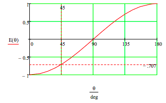
If the observers measure their spins in the same direction (both θ = 0 deg or both θ = 45 deg) quantum mechanics predicts they will get opposite values due to the singlet nature of the spin state. In other words, the combined expectation value is -1 for these measurements as shown in the figure above. However, if they measure their spins at 0 and 45 degrees, the expectation value is -0.707.

Realists believe that objects have well-defined properties prior to and independent of observation. Specific 0- and 45-deg spin states are assigned to the particles in the first two columns, with each particle in one of four equally probable spin orientations consistent with the composite singlet state. The next two columns show that these assignments agree with the quantum predictions when both spins are measured at the same angle. The last column shows that these spin assignments disagree with the quantum prediction when one spin is measured at 0 degrees and the other at 45 degrees.

\[ \begin{bmatrix} \text{Particle A} & \text{Particle B} & \hat{S}_0 \text{(A)} \hat{S}_0 \text{(B)} & \hat{S}_{45} \text{(A)} \hat{S}_{45} \text{(B)} & \hat{S}_0 \text{(A)} \hat{S}_{45} \text{(B)} \\ | \uparrow \rangle | \nearrow \rangle & | \downarrow \rangle | \swarrow \rangle & -1 & -1 & -1 \\ | \uparrow \rangle | \swarrow \rangle & | \downarrow \rangle | \nearrow \rangle & -1 & -1 & 1 \\ | \downarrow \rangle | \nearrow \rangle & | \uparrow \rangle | \swarrow \rangle & -1 & -1 & 1 \\ | \downarrow \rangle | \swarrow \rangle & | \uparrow \rangle | \nearrow \rangle & -1 & -1 & -1 \\ \text{Realist} & \text{Value} & -1 & -1 & 0 \\ \text{Quantum} & \text{Value} & -1 & -1 & -0.707 \end{bmatrix} \nonumber \]

This brief analysis demonstrates that there are conceptually simple, Stern-Gerlach like, experiments on spin-1/2 systems which can adjudicate the conflict between local realism and quantum mechanics.

In addition to the disagreement shown in the last column of the table, quantum theory asserts that the realist's spin states are invalid. The spin operator at an angel θ to the vertical in the xz-plane is

\[ \text{Op} ( \theta) = \varphi_u ( \theta)^T \varphi_d ( \theta) - \varphi_d ( \theta) \varphi_d ( \theta)^T \text{ simplify } \rightarrow \begin{pmatrix} \cos ( \theta) & \sin ( \theta) \\ \sin ( \theta) & - \cos ( \theta) \end{pmatrix} \nonumber \]

The operators for spin measurements at 0 and 45 degrees in the xz-plane do not commute.

\[ \text{Op (0 deg) Op(45 deg)} - \text{Op(45 deg) Op(0 deg)} = \begin{pmatrix} 0 & 1.414 \\ -1.414 & 0 \end{pmatrix} \nonumber \]

Therefore, according to quantum theory a particle's spin cannot be simultaneously well-defined for both 0 and 45 degrees.

Addendum

According to Richard Feynman it takes a quantum computer to simulate quantum pheonomenon. The following quantum circuit produces results that are in agreement with experiment as summarized in the graph above. The Hadamard and CNOT gates create the singlet state from the |11> input. R_z(θ) is the rotation of the measuring device of the second spin. The final Hadamard gates prepare the system for measurement in the x-basis. See arXiv:1712.05642v2 for further detail.

\[ \begin{matrix} |1 \rangle & \triangleright & \text{H} & \cdot & \cdots & \text{H} & \triangleright & \text{Measure 0 or 1} \\ ~ & ~ & ~ & | \\ |1 \rangle & \triangleright & \cdots & \oplus & \text{R}_z( \theta) & \text{H} & \triangleright & \text{Measure 0 or 1} \end{matrix} \nonumber \]

The quantum operators required to execute this circuit are:

\[ \begin{matrix} \text{I} = \begin{pmatrix} 1 & 0 \\ 0 & 1 \end{pmatrix} & \text{H} = \frac{1}{ \sqrt{2}} \begin{pmatrix} 1 & 1 \\ 1 & -1 \end{pmatrix} & \text{R}_z ( \theta) = \begin{pmatrix} 1 & 0 \\ 0 & e^{i \theta} \end{pmatrix} & \text{CNOT} = \begin{pmatrix} 1 & 0 & 0 & 0 \\ 0 & 1 & 0 & 0 \\ 0 & 0 & 0 & 1 \\ 0 & 0 & 1 & 0 \end{pmatrix} \end{matrix} \nonumber \]

\[ \text{BellCircuit} ( \theta) = \text{kronecker(H, H) kronecker} \left( \text{(I, R)}_z ( \theta) \right) \text{CNOT kronecker(H, I)} \nonumber \]

The circuit is run for θ = π/4 to demonstrate that it produces the result highlighted in the graph above. In addition, by varying θ it can be shown that the circuit reproduces the entire plot of E(θ). There are four output states shown below. If the spins are measured in the same state, |00> or |11>, the eigenvalue is +1, if they are different, |01> or |10>, the eigenvalue is -1. The probability for each output state is calculated on the right.

\[ \begin{matrix} \text{Output state} & \text{Eigenvalue} & \text{Probability} \\ | 00 \rangle = \begin{pmatrix} 1 \\ 0 \end{pmatrix} \otimes \begin{pmatrix} 1 \\ 0 \end{pmatrix} = \begin{pmatrix} 1 \\ 0 \\ 0 \\ 0 \end{pmatrix} & 1 & \left[ \left| \begin{pmatrix} 1 \\ 0 \\ 0 \\ 0 \end{pmatrix}^T \text{BellCircuit} \left( \frac{ \pi}{4} \right) \begin{pmatrix} 0 \\ 0 \\ 0 \\ 1 \end{pmatrix} \right| \right]^2 = 0.0732 \\ | 01 \rangle = \begin{pmatrix} 1 \\ 0 \end{pmatrix} \otimes \begin{pmatrix} 0 \\ 1 \end{pmatrix} = \begin{pmatrix} 0 \\ 1 \\ 0 \\ 0 \end{pmatrix} & -1 & \left[ \left| \begin{pmatrix} 0 \\ 1 \\ 0 \\ 0 \end{pmatrix}^T \text{BellCircuit} \left( \frac{ \pi}{4} \right) \begin{pmatrix} 0 \\ 0 \\ 0 \\ 1 \end{pmatrix} \right| \right]^2 = 0.4268 \\ | 10 \rangle = \begin{pmatrix} 0 \\ 1 \end{pmatrix} \otimes \begin{pmatrix} 1 \\ 0 \end{pmatrix} = \begin{pmatrix} 0 \\ 0 \\ 1 \\ 0 \end{pmatrix} & -1 & \left[ \left| \begin{pmatrix} 0 \\ 0 \\ 1 \\ 0 \end{pmatrix}^T \text{BellCircuit} \left( \frac{ \pi}{4} \right) \begin{pmatrix} 0 \\ 0 \\ 0 \\ 1 \end{pmatrix} \right| \right]^2 = 0.4268 \\ |11 \rangle = \begin{pmatrix} 0 \\ 1 \end{pmatrix} \otimes \begin{pmatrix} 0 \\ 1 \end{pmatrix} = \begin{pmatrix} 0 \\ 0 \\ 0 \\ 1 \end{pmatrix} & 1 & \left[ \left| \begin{pmatrix} 0 \\ 0 \\ 0 \\ 1 \end{pmatrix}^T \text{BellCircuit} \left( \frac{ \pi}{4} \right) \begin{pmatrix} 0 \\ 0 \\ 0 \\ 1 \end{pmatrix} \right| \right]^2 = 0.0732 \end{matrix} \nonumber \]

Expectation value or correlation coeficient:

\[ 0.0732 - 0.4268 - 0.4268 + 0.0732 = -0.707 \nonumber \]

A classical computer manipulates bits which are in well-defined states consisting of 0s and 1s.This entangled two-spin experiment demonstrates that simulation of quantum physics requires a computer that can manipulate 0s and 1s, superpositions of 0 and 1, and entangled superpositions of 0s and 1s. Simulation of quantum physics requires a quantum computer, and the circuit shown above is a quantum computer.

An alternative computational method using projection operators:

\[ \begin{matrix} \text{Output state} & \text{Eigenvalue} & \text{Probability} \\ | 00 \rangle = \begin{pmatrix} 1 \\ 0 \end{pmatrix} \otimes \begin{pmatrix} 1 \\ 0 \end{pmatrix} = \begin{pmatrix} 1 \\ 0 \\ 0 \\ 0 \end{pmatrix} & 1 & \left[ \left| \text{kronecker} \left[ \begin{pmatrix} 1 & 0 \\ 0 & 0 \end{pmatrix},~ \begin{pmatrix} 1 & 0 \\ 0 & 0 \end{pmatrix} \right] \text{BellCircuit} \left( \frac{ \pi}{4} \right) \begin{pmatrix} 0 \\ 0 \\ 0 \\ 1 \end{pmatrix} \right| \right]^2 = 0.0732 \\ | 01 \rangle = \begin{pmatrix} 1 \\ 0 \end{pmatrix} \otimes \begin{pmatrix} 0 \\ 1 \end{pmatrix} = \begin{pmatrix} 0 \\ 1 \\ 0 \\ 0 \end{pmatrix} & -1 & \left[ \left|\text{kronecker} \left[ \begin{pmatrix} 1 & 0 \\ 0 & 0 \end{pmatrix},~ \begin{pmatrix} 0 & 0 \\ 0 & 1 \end{pmatrix} \right] \text{BellCircuit} \left( \frac{ \pi}{4} \right) \begin{pmatrix} 0 \\ 0 \\ 0 \\ 1 \end{pmatrix} \right| \right]^2 = 0.4268 \\ | 10 \rangle = \begin{pmatrix} 0 \\ 1 \end{pmatrix} \otimes \begin{pmatrix} 1 \\ 0 \end{pmatrix} = \begin{pmatrix} 0 \\ 0 \\ 1 \\ 0 \end{pmatrix} & -1 & \left[ \left| \text{kronecker} \left[ \begin{pmatrix} 0 & 0 \\ 0 & 1 \end{pmatrix},~ \begin{pmatrix} 1 & 0 \\ 0 & 0 \end{pmatrix} \right] \text{BellCircuit} \left( \frac{ \pi}{4} \right) \begin{pmatrix} 0 \\ 0 \\ 0 \\ 1 \end{pmatrix} \right| \right]^2 = 0.4268 \\ |11 \rangle = \begin{pmatrix} 0 \\ 1 \end{pmatrix} \otimes \begin{pmatrix} 0 \\ 1 \end{pmatrix} = \begin{pmatrix} 0 \\ 0 \\ 0 \\ 1 \end{pmatrix} & 1 & \left[ \left| \text{kronecker} \left[ \begin{pmatrix} 0 & 0 \\ 0 & 1 \end{pmatrix},~ \begin{pmatrix} 0 & 0 \\ 0 & 1 \end{pmatrix} \right] \text{BellCircuit} \left( \frac{ \pi}{4} \right) \begin{pmatrix} 0 \\ 0 \\ 0 \\ 1 \end{pmatrix} \right| \right]^2 = 0.0732 \end{matrix} \nonumber \]

Measuring only one spin using a projection operator and the identity:

\[ \begin{matrix} \left[ \left| \text{kronecker} \left[ \begin{pmatrix} 1 & 0 \\ 0 & 0 \end{pmatrix},~ \begin{pmatrix} 1 & 0 \\ 0 & 1 \end{pmatrix} \right] \text{BellCircuit} \left( \frac{ \pi}{4} \right) \begin{pmatrix} 0 \\ 0 \\ 0 \\ 1 \end{pmatrix} \right| \right]^2 = 0.5 & \left[ \left|\text{kronecker} \left[ \begin{pmatrix} 0 & 0 \\ 0 & 1 \end{pmatrix},~ \begin{pmatrix} 1 & 0 \\ 0 & 1 \end{pmatrix} \right] \text{BellCircuit} \left( \frac{ \pi}{4} \right) \begin{pmatrix} 0 \\ 0 \\ 0 \\ 1 \end{pmatrix} \right| \right]^2 = 0.5 \\ \left[ \left|\text{kronecker} \left[ \begin{pmatrix} 1 & 0 \\ 0 & 1 \end{pmatrix},~ \begin{pmatrix} 1 & 0 \\ 0 & 0 \end{pmatrix} \right] \text{BellCircuit} \left( \frac{ \pi}{4} \right) \begin{pmatrix} 0 \\ 0 \\ 0 \\ 1 \end{pmatrix} \right| \right]^2 = 0.5 & \left[ \left| \text{kronecker} \left[ \begin{pmatrix} 1 & 0 \\ 0 & 1 \end{pmatrix},~ \begin{pmatrix} 0 & 0 \\ 0 & 1 \end{pmatrix} \right] \text{BellCircuit} \left( \frac{ \pi}{4} \right) \begin{pmatrix} 0 \\ 0 \\ 0 \\ 1 \end{pmatrix} \right| \right]^2 = 0.5 \end{matrix} \nonumber \]