7.31: Quantum Correlations Illuminated with Tensor Algebra

Jim Baggott’s excellent text, The Meaning of Quantum Theory, deals with the fundamentals of quantum mechanics and its various philosophical interpretations. His demonstrations of computational methods (generally using Dirac algebra) are easy to follow and his summaries of the interpretive positions of Bohr, Einstein, Bohm, Everett, etc. are lucid. Of special note is the clarity with which he deals with the importance of the work of John S. Bell and the eponymous Bell’s theorem.

In order to appreciate the significance of Bell’s theorem you need to be willing to do some math. This tutorial deals with recasting the mathematics of Baggott’s treatment of quantum correlations (pages 119 to 127) using tensor algebra. Not because there is any deficiency in his math, but simply to present another, related method.

The experiment analyzed involves the simultaneous release of two entangled photons in opposite directions as shown below, followed by measurement of their polarization state in the vertical/horizontal measurement basis. The experimental set‐up allows for the rotation of the right‐hand detector through an angle of Θ, in order to more thoroughly explore the consequences of photon entanglement.

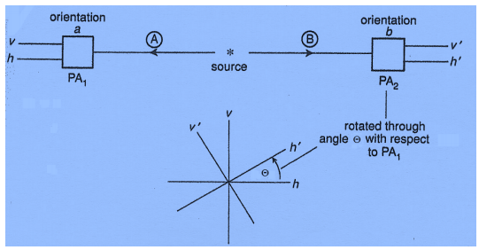
The experiment involves measurement of the polarization states of the photon pairs (A,B) as diagramed above. The various polarization states involved are presented below in vector notation: v = vertical; h = horizontal; L = left circular; R = right circular.

\[ |v \rangle = \begin{pmatrix} 1 \\ 0 \end{pmatrix} \nonumber \]

\[ |v' \rangle = \begin{pmatrix} \cos \theta \\ - \sin \theta \end{pmatrix} \nonumber \]

\[ |v \rangle = \begin{pmatrix} 0 \\ 1 \end{pmatrix} \nonumber \]

\[ |h' \rangle = \begin{pmatrix} \sin \theta \\ \cos \theta \end{pmatrix} \nonumber \]

\[ | L \rangle = \frac{1}{ \sqrt{2}} \begin{pmatrix} 1 \\ i \end{pmatrix} \nonumber \]

\[ | R \rangle = \frac{1}{ \sqrt{2}} \begin{pmatrix} 1 \\ -i \end{pmatrix} \nonumber \]

The initial state (see Baggott for details) is the following entangled superposition. In other words, both photons, the one moving to the right and the one moving to the left are in the same circular polarization state.

\[ | \Psi \rangle = \frac{1}{ \sqrt{2}} \left[ |L \rangle_A |L \rangle_B + |R \rangle_A |R \rangle_B \right] \nonumber \]

This initial photon state is recast using the vector tensor product, which is formed as follows.

\[ \begin{pmatrix} a \\ b \end{pmatrix} \otimes \begin{pmatrix} c \\ d \end{pmatrix} = \begin{pmatrix} ac \\ ad \\ bc \\ bd \end{pmatrix} \nonumber \]

Therefore in the tensor format the initial state is,

\[ | \Psi \rangle = \frac{1}{ \sqrt{2}} \left[ |L \rangle_A |L \rangle_B + |R \rangle_A |R \rangle_B \right] = \frac{1}{2 \sqrt{2}} \left[ \begin{pmatrix} 1 \\ i \end{pmatrix}_A \otimes \begin{pmatrix} 1 \\ i \end{pmatrix}_B + \begin{pmatrix} 1 \\ -i \end{pmatrix}_A \otimes \begin{pmatrix} 1 \\ -i \end{pmatrix}_B \right] = \frac{1}{ 2 \sqrt{2}} \left[ \begin{pmatrix} 1 \\ i \\ i \\ -1 \end{pmatrix} + \begin{pmatrix} 1 \\ -i \\ -i \\ -1 \end{pmatrix} \right] = \frac{1}{ \sqrt{2}} \begin{pmatrix} 1 \\ 0 \\ 0 \\ -1 \end{pmatrix} \nonumber \]

There are four measurement outcomes for the photon pairs. Both photons can be detected in the vertical state, both in the horizontal state, A in the vertical state and B in the horizontal state, and vice versa. The measurement eigenstates are calculated below in tensor format.

\[ \psi '_{vv} \rangle = | v \rangle_A |v' \rangle_B = \begin{pmatrix} 1 \\ 0 \end{pmatrix} \otimes \begin{pmatrix} \cos \theta \\ - \sin \theta \end{pmatrix} = \begin{pmatrix} \cos \theta \\ - \sin \theta \\ 0 \\ 0 \end{pmatrix} \nonumber \]

\[ \psi '_{vh} \rangle = | v \rangle_A |h' \rangle_B = \begin{pmatrix} 1 \\ 0 \end{pmatrix} \otimes \begin{pmatrix} \sin \theta \\ \cos \theta \end{pmatrix} = \begin{pmatrix} \sin \theta \\ \cos \theta \\ 0 \\ 0 \end{pmatrix} \nonumber \]

\[ \psi '_{hv} \rangle = | h \rangle_A |v' \rangle_B = \begin{pmatrix} 0 \\ 1 \end{pmatrix} \otimes \begin{pmatrix} \cos \theta \\ - \sin \theta \end{pmatrix} = \begin{pmatrix} 0 \\ 0 \\ \cos \theta \\ - \sin \theta \end{pmatrix} \nonumber \]

\[ \psi '_{hh} \rangle = | h \rangle_A |h' \rangle_B = \begin{pmatrix} 0 \\ 1 \end{pmatrix} \otimes \begin{pmatrix} \sin \theta \\ \cos \theta \end{pmatrix} = \begin{pmatrix} 0 \\ 0 \\ \sin \theta \\ \cos \theta \end{pmatrix} \nonumber \]

The probability amplitudes for these experimental possibilities are found by calculating the projection of their eigenstates onto the initial state vector.

\[ \langle \psi '_{vv} | \Psi \rangle \begin{pmatrix} \cos \theta & - \sin \theta & 0 & 0 \end{pmatrix} \frac{1}{ \sqrt{2}} \begin{pmatrix} 1 \\ 0 \\ 0 \\ -1 \end{pmatrix} = \frac{1}{ \sqrt{2}} \cos \theta \nonumber \]

\[ \langle \psi '_{vh} | \Psi \rangle \begin{pmatrix} \sin \theta & \cos \theta & 0 & 0 \end{pmatrix} \frac{1}{ \sqrt{2}} \begin{pmatrix} 1 \\ 0 \\ 0 \\ -1 \end{pmatrix} = \frac{1}{ \sqrt{2}} \sin \theta \nonumber \]

\[ \langle \psi '_{hv} | \Psi \rangle \begin{pmatrix} 0 & 0 & \cos \theta & - \sin \theta \end{pmatrix} \frac{1}{ \sqrt{2}} \begin{pmatrix} 1 \\ 0 \\ 0 \\ -1 \end{pmatrix} = \frac{1}{ \sqrt{2}} \sin \theta \nonumber \]

\[ \langle \psi '_{hh} | \Psi \rangle \begin{pmatrix} 0 & 0 & \sin \theta & \cos \theta \end{pmatrix} \frac{1}{ \sqrt{2}} \begin{pmatrix} 1 \\ 0 \\ 0 \\ -1 \end{pmatrix} = - \frac{1}{ \sqrt{2}} \cos \theta \nonumber \]

This yields the following probabilities for the four experimental outcomes. (See Baggott’s equation 4.16 on page 127 of his text.)

\[ P_{vv} ( \theta ) = \left| \langle \psi '_{vv} | \Psi \rangle \right|^2 = \frac{1}{2} \cos^2 \theta \nonumber \]

\[ P_{vh} ( \theta ) = \left| \langle \psi '_{vh} | \Psi \rangle \right|^2 = \frac{1}{2} \sin^2 \theta \nonumber \]

\[ P_{hv} ( \theta ) = \left| \langle \psi '_{hv} | \Psi \rangle \right|^2 = \frac{1}{2} \sin^2 \theta \nonumber \]

\[ P_{hh} ( \theta ) = \left| \langle \psi '_{hh} | \Psi \rangle \right|^2 = \frac{1}{2} \cos^2 \theta \nonumber \]

(Note that if Θ = 0, we get the results Baggott reports on page 122.)

Baggott goes on to show how this experiment and its more sophisticated successors, and their quantum mechanical analyses, illuminate the contradiction between the quantum and classical visions of reality. The purpose of this tutorial has been merely to present a somewhat different format for carrying out the quantum mechanical calculations.