7.25: A Quantum Optical Cheshire Cat

The following is a summary of "Quantum Cheshire Cats" by Aharonov, Popescu, Rohrlich and Skrzypczyk which was published in the New Journal of Physics 15, 113015 (2013) and can also be accessed at: arXiv:1202.0631v2.

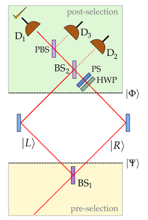
In the absence of the half-wave plate (HWP) and the phase shifter (PS) a horizontally polarized photon entering the interferometer from the lower left (propagating to the upper right) arrives at D₂ with a 90 degree (π/2, i) phase shift. (By convention reflection at a beam splitter introduces a 90 degree phase shift.)

\[ |R \rangle |H \rangle \xrightarrow{BS_1} \frac{1}{ \sqrt{2}} [ i | L \rangle + |R \rangle ] |H \rangle \xrightarrow{BS_2} i | D_2 \rangle | H \rangle \nonumber \]

The state immediately after the first beam splitter is the pre-selected state.

\[ | Psi \rangle = \frac{1}{ \sqrt{2}} \left[ i | L \rangle + | R \rangle \right] |H \rangle \nonumber \]

The post-selected state is,

\[ | \Phi \rangle = \frac{1}{ \sqrt{2}} \left[ | L \rangle |H \rangle + | R \rangle |V \rangle \right] \nonumber \]

The HWP (converts |V> to |H> in the R-branch) and PS transform this state to,

\[ | \Phi \rangle \xrightarrow[PS]{HWP} \frac{1}{ \sqrt{2}} \left[ | L \rangle + i | R \rangle \right] |H \rangle \nonumber \]

which exits the second beam splitter through the left port to encounter a polarizing beam splitter which transmits horizontal polarization and reflects vertical polarization. Thus, the post-selected state is detected at D₁. The evolution of the post-selected state is summarized as follows:

\[ | \Phi \rangle = \frac{1}{ \sqrt{2}} \left[ |L \rangle |H \rangle + |R \rangle |V \rangle \right] \xrightarrow[PS]{HWP} \frac{1}{ \sqrt{2}} \left[ | L \rangle + i | R \rangle \right] |H \rangle \xrightarrow{BS_2} i |L \rangle |H \rangle \xrightarrow{PBS} i | D_1 \rangle |H \rangle \nonumber \]

The last term on the right side below is the weak value of A multiplied by the probability of its occurrence for the preselected state Ψ and the post-selected state Φ.

\[ \langle \Psi | \hat{A} | \Psi \rangle = \sum_j \langle \Psi | \Phi_j \rangle \langle \Phi_j | \hat{A} | \Psi \rangle = \sum_j \langle \Psi | \Phi_j \rangle \langle \Phi_j | \Psi \rangle \frac{ \langle \Phi_j | \hat{A} | \Psi \rangle}{ \langle \Phi_j | \Psi \rangle} = \sum_j p_j \frac{ \langle \Phi_j | \hat{A} | \Psi \rangle}{ \langle \Phi_j | \Psi \rangle} \nonumber \]

The weak value calculations are carried out in a 4-dimensional Hilbert space created by the tensor product of the photon's direction of propagation and polarization vectors.

Direction of propagation vectors:

\[ L = \begin{pmatrix} 1 \\ 0 \end{pmatrix} \nonumber \]

\[ R = \begin{pmatrix} 0 \\ 1 \end{pmatrix} \nonumber \]

Polarization state vectors:

\[ H = \begin{pmatrix} 1 \\ 0 \end{pmatrix} \nonumber \]

\[ V = \begin{pmatrix} 0 \\ 1 \end{pmatrix} \nonumber \]

Pre-selected state:

\[ \Psi = \frac{1}{ \sqrt{2}} (iL + R)H = \frac{1}{ \sqrt{2}} \left[ i \begin{pmatrix} 1 \\ 0 \end{pmatrix} + \begin{pmatrix} 0 \\ 1 \end{pmatrix} \right] + \begin{pmatrix} 1 \\ 0 \end{pmatrix} = frac{1}{ \sqrt{2}} \begin{pmatrix} i \\ 1 \end{pmatrix} \begin{pmatrix} 1 \\ 0 \end{pmatrix} \nonumber \]

\[ \Psi = \frac{1}{ \sqrt{2}} \begin{pmatrix} i \\ 0 \\ 1 \\ 0 \end{pmatrix} \nonumber \]

Post-selected state:

\[ \Phi = \frac{1}{ \sqrt{2}} (LH + RV) = \frac{1}{ \sqrt{2}} \left[ \begin{pmatrix} 1 \\ 0 \end{pmatrix} + \begin{pmatrix} 1 \\ 0 \end{pmatrix} + \begin{pmatrix} 0 \\ 1 \end{pmatrix} + \begin{pmatrix} 0 \\ 1 \end{pmatrix} \right] \nonumber \]

\[ \Phi = \frac{1}{ \sqrt{2}} \begin{pmatrix} 1 \\ 0 \\ 0 \\ 1 \end{pmatrix} \nonumber \]

Direction of propagation operators:

\[ Left = \begin{pmatrix} 1 \\ 0 \end{pmatrix} \begin{pmatrix} 1 & 0 \end{pmatrix} \rightarrow \begin{pmatrix} 1 & 0 \\ 0 & 0 \end{pmatrix} \nonumber \]

\[ Right = \begin{pmatrix} 0 \\ 1 \end{pmatrix} \begin{pmatrix} 0 & 1 \end{pmatrix} \rightarrow \begin{pmatrix} 0 & 0 \\ 0 & 1 \end{pmatrix} \nonumber \]

Photon angular momentum operator:

\[ Pang = \begin{pmatrix} 0 & -i \\ i & 0 \end{pmatrix} \nonumber \]

Identity operator:

\[ I = \begin{pmatrix} 1 & 0 \\ 0 & 1 \end{pmatrix} \nonumber \]

The following weak value calculations show that for the pre- and post-selection ensemble of observations the photon is in the left arm of the interferometer while its angular momentum is in the right arm. Like the case of the Cheshire cat, a photon property has been separated from the photon.

\[ \begin{pmatrix} "" & "Left ~Arm" & "Right ~Arm" \\ "Arm" & \frac{ \Phi^T kronecker(Left, ~I) \Psi}{ \Phi^T \Psi} & \frac{ \Phi^T kronecker(Right, ~I) \Psi}{ \Phi^T \Psi} \\ "Pang" & \frac{ \Phi^T kronecker(Left, ~Pang) \Psi}{ \Phi^T \Psi} & \frac{ \Phi^T kronecker(Right, ~Pang) \Psi}{ \Phi^T \Psi} \end{pmatrix} = \begin{pmatrix} "" & "Left~Arm" & "Right~Arm \\ "Arm" & 1 & 0 \\ "Pang" & 0 & 1 \end{pmatrix} \nonumber \]

The following shows the evolution of the pre-selected state to the final state at the detectors. The intermediate is the state illuminating BS₂. The polarization state at the detectors is ignored.

\[ | \Psi \rangle \rightarrow \frac{i}{ \sqrt{2}} \left[ |L \rangle |H \rangle + |R \rangle |V \rangle \right] \rightarrow - \frac{1}{2} |D_1 \rangle + \frac{i}{2} | D_3 \rangle + \frac{(i-1)}{2} |D_2 \rangle \nonumber \]

Squaring the magnitude of the probability amplitudes shows that the probabilities that D₁, D₃ and D₂ will fire are 1/4, 1/4 and 1/2, respectively. The probability at D₁ is consistent with the probability that the post-selected state is contained in the pre-selected state. A photon in the post-selected state has a probability of 1 of reaching D₁ and it represents a 25% contribution to the pre-selected state.

\[ (| \Phi^T \Psi |)^2 \rightarrow \frac{1}{4} \nonumber \]

Note that the expectation values for the pre-selected state show no path-polarization separation.

\[ \begin{pmatrix} "" & "Left~Arm" & "Right~Arm" \\ "Arm" & ( \overline{ \Psi})^T kronecker(Left,~I) \Psi & ( \overline{ \Psi})^T kronecker(Right,~I) \Psi \\ "Pang" & ( \overline{ \Psi})^T kronecker(Left,~Pang) \Psi & ( \overline{ \Psi})^T kronecker(Right,~Pang) \Psi \\ "Hop" & ( \overline{ \Psi})^T kronecker(Left,~HH^T) \Psi & ( \overline{ \Psi})^T kronecker(Right,~HH^T) \Psi \\ "Vop" & ( \overline{ \Psi})^T kronecker(Left,~VV^T) \Psi & ( \overline{ \Psi})^T kronecker(Right,~VV^T) \Psi \end{pmatrix} = \begin{pmatrix} "" & "Left~Arm" & "Right~Arm" \\ "Arm" & 0.5 & 0.5 \\ "Pang" & 0 & 0 \\ "Hop" & 0.5 & 0.5 \\ "Vop" & 0 & 0 \end{pmatrix} \nonumber \]

In addition the following table shows that linear polarization (HV) is not separated from the photon's path.

\[ HV = \begin{pmatrix} 1 & 0 \\ 0 & -1 \end{pmatrix} \nonumber \]

\[ \begin{pmatrix} "" & "Left ~Arm" & "Right ~Arm" \\ "Arm" & \frac{ \Phi^T kronecker(Left, ~I) \Psi}{ \Phi^T \Psi} & \frac{ \Phi^T kronecker(Right, ~I) \Psi}{ \Phi^T \Psi} \\ "HV" & \frac{ \Phi^T kronecker(Left, ~HV) \Psi}{ \Phi^T \Psi} & \frac{ \Phi^T kronecker(Right, ~HV) \Psi}{ \Phi^T \Psi} \end{pmatrix} = \begin{pmatrix} "" & "Left~Arm" & "Right~Arm \\ "Arm" & 1 & 0 \\ "HV" & 1 & 0 \end{pmatrix} \nonumber \]

The "Complete Quantum Cheshire Cat" by Guryanova, Brunner and Popescu (arXiv 1203.4215) provides an optical set-up which achieves complete path-polarization separation for the photon.