1.12: Quantum Computation- A Short Course

Quantum Correlations Illustrated With Spin-1/2 Particles

A spin-1/2 pair is prepared in an entangled singlet state and the individual particles travel in opposite directions on the y-axis to a pair of Stern-Gerlach detectors which are set up to measure spin in the x-z plane. Particle A's spin is measured along the z-axis, and particle B's spin is measured at an angle \(\theta\) with respect to the z-axis.

Spin-up eigenstate Eigenvalue +1 \[ \varphi_{\mathrm{u}}(\theta)=\left( \begin{array}{c}{\cos \left(\frac{\theta}{2}\right)} \\ {\sin \left(\frac{\theta}{2}\right)}\end{array}\right) \nonumber \]

Spin-down eigenstate Eigenvalue -1 \[ \varphi_{\mathrm{d}}(\theta) :=\left( \begin{array}{c}{-\sin \left(\frac{\theta}{2}\right)} \\ {\cos \left(\frac{\theta}{2}\right)}\end{array}\right) \nonumber \]

The singlet state wave function in the xz-plane:

\[
| \Psi \rangle=\frac{1}{\sqrt{2}}[ |\uparrow\rangle_{\mathrm{A}} | \downarrow \rangle_{\mathrm{B}}-| \downarrow \rangle_{\mathrm{A}} | \uparrow \rangle_{\mathrm{B}} ] =\frac{1}{\sqrt{2}}\left[\left( \begin{array}{c}{\cos \left(\frac{\theta}{2}\right)} \\ {\sin \left(\frac{\theta}{2}\right)}\end{array}\right)_{A} \otimes \left( \begin{array}{c}{-\sin \left(\frac{\theta}{2}\right)} \\ {\cos \left(\frac{\theta}{2}\right)}\end{array}\right)_{B}-\left( \begin{array}{c}{-\sin \left(\frac{\theta}{2}\right)} \\ {\cos \left(\frac{\theta}{2}\right)}\end{array}\right)_{A} \otimes \left( \begin{array}{c}{\cos \left(\frac{\theta}{2}\right)} \\ {\sin \left(\frac{\theta}{2}\right)}\end{array}\right)_{B}\right] =\frac{1}{\sqrt{2}} \left( \begin{array}{c}{0} \\ {1} \\ {-1} \\ {0}\end{array}\right)
\nonumber \]

The spin operator in the \(\theta\) direction:

\[
\mathrm{S}(\theta) :=\varphi_{\mathrm{u}}(\theta) \cdot \varphi_{\mathrm{u}}(\theta)^{\mathrm{T}}-\varphi_{\mathrm{d}}(\theta) \cdot \varphi_{\mathrm{d}}(\theta)^{\mathrm{T}} \text { simplify } \rightarrow \left( \begin{array}{cc}{\cos (\theta)} & {\sin (\theta)} \\ {\sin (\theta)} & {-\cos (\theta)}\end{array}\right)
\nonumber \]

\[
\sigma_{\mathrm{Z}} :=\left( \begin{array}{cc}{1} & {0} \\ {0} & {-1}\end{array}\right) \quad \sigma_{\mathrm{X}}=\left( \begin{array}{ll}{0} & {1} \\ {1} & {0}\end{array}\right) \quad \mathrm{S}(\theta) :=\cos (\theta) \cdot \sigma_{\mathrm{Z}}+\sin (\theta) \cdot \sigma_{\mathrm{x}} \rightarrow \left( \begin{array}{cc}{\cos (\theta)} & {\sin (\theta)} \\ {\sin (\theta)} & {-\cos (\theta)}\end{array}\right)
\nonumber \]

The composite spin operator in the z-direction for A and at an angle θ in the xz-plane for B.

\[
S(0) \otimes S(\theta)=\left( \begin{array}{cc}{1} & {0} \\ {0} & {-1}\end{array}\right) \otimes \left( \begin{array}{cc}{\cos \theta} & {\sin \theta} \\ {\sin \theta} & {-\cos \theta}\end{array}\right)=\left( \begin{array}{cccc}{\cos \theta} & {\sin \theta} & {0} & {0} \\ {\sin \theta} & {-\cos \theta} & {0} & {0} \\ {0} & {0} & {-\cos \theta} & {-\sin \theta} \\ {0} & {0} & {-\sin \theta} & {\cos \theta}\end{array}\right)
\nonumber \]

Calculate and display the expectation value or correlation coefficient.

\[
\Psi_{m} :=\frac{1}{\sqrt{2}} \left( \begin{array}{c}{0} \\ {1} \\ {-1} \\ {0}\end{array}\right)
\nonumber \]

\[
E(\theta) :=\Psi_{m}^{T} \left( \begin{array}{cccc}{\cos (\theta)} & {\sin (\theta)} & {0} & {0} \\ {\sin (\theta)} & {-\cos (\theta)} & {0} & {0} \\ {0} & {0} & {-\cos (\theta)} & {-\sin (\theta)} \\ {0} & {0} & {-\sin (\theta)} & {\cos (\theta)}\end{array}\right) \cdot \Psi_{m} \rightarrow-\cos (\theta)
\nonumber \]

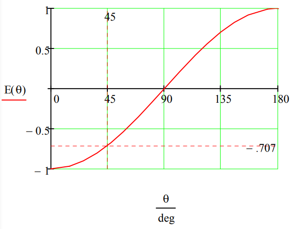
Demonstrate that a hidden-value model that assigns spin orientations in non-orthogonal directions to A and B disagrees with the quantum calculation at 45 degrees.

\[\left[ \begin{matrix} \text{Particle A} & \text{Particle B} & \hat{S}_{0}(\mathrm{A}) \cdot \hat{S}_{0}(\mathrm{B}) & \hat{S}_{45}(\mathrm{A}) \cdot \hat{S}_{45}(\mathrm{B}) & \hat{S}_{0}(\mathrm{A}) \cdot \hat{S}_{45}(\mathrm{B}) \\ | \uparrow \rangle | \nearrow \rangle & | \downarrow \rangle | \swarrow \rangle & -1 & -1 & -1 \\ | \uparrow \rangle | \swarrow \rangle & | \downarrow \rangle | \nearrow \rangle & -1 & -1 & 1 \\ | \downarrow \rangle | \nearrow \rangle & | \uparrow \rangle | \swarrow \rangle & -1 & -1 & 1 \\ | \downarrow \rangle | \swarrow \rangle & | \uparrow \rangle | \nearrow \rangle & -1 & -1 & -1 \\ \text{Realist} & \text{Value} & -1 & -1 & 0 \\ \text{Quantum} & \text{Value} & -1 & -1 & -0.707 \end{matrix} \right] \nonumber \]

Quantum Correlations Illustrated With Photons

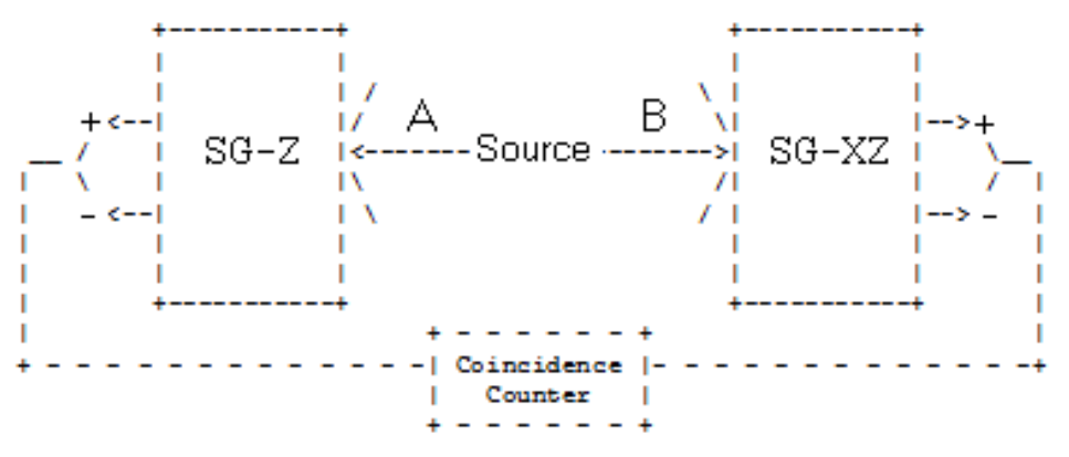
A two-stage atomic cascade emits entangled photons (A and B) in opposite directions with the same circular polarization according to observers in their path. The experiment involves the measurement of photon polarization states in the vertical/horizontal measurement basis, and allows for the rotation of the right-hand detector through an angle of \(\theta\), in order to explore the consequences of quantum mechanical entanglement. PA stands for polarization analyzer and could simply be a calcite crystal.

\[\begin{matrix} V & \lhd & \lceil & \; & \rceil & \; & \; & \; & \lceil & \; & \rceil & \rhd & V \\ \; & \; & | & 0 & | & \xleftarrow{A} & \xleftrightarrow{Source} & \xrightarrow{B} & | & \theta & | & \; & \; \\ H & \lhd & \lfloor & \; & \rfloor & \; & \; & \; & \lfloor & \; & \rfloor & \rhd & H \\ \; & \; & \; & PA_{A} & \; & \; & \; & \; & \; & PA_{B} & \; & \; & \; \end{matrix} \nonumber \]

\[
| \Psi \rangle=\frac{1}{\sqrt{2}}[ |L\rangle_{A} | L \rangle_{B}+| R \rangle_{A} | R \rangle_{B} ]=\frac{1}{\sqrt{2}}[ |V\rangle_{A} | V \rangle_{B}-| H \rangle_{A} | H \rangle_{B} ]=\frac{1}{\sqrt{2}} \left( \begin{array}{l}{1} \\ {0} \\ {0} \\ {-1}\end{array}\right)
\nonumber \]

using

\[
| L \rangle=\frac{1}{\sqrt{2}}[ |V\rangle+ i | H \rangle ] \quad | R \rangle=\frac{1}{\sqrt{2}}[ |V\rangle- i | H \rangle ]
\nonumber \]

Calculate the composite polarization measurement operator for 0 degrees (A) and \(\theta\) degrees (B):

\[
\mathrm{V}(\theta) :=\left( \begin{array}{l}{\cos (\theta)} \\ {\sin (\theta)}\end{array}\right) \quad H(\theta) :=\left( \begin{array}{c}{-\sin (\theta)} \\ {\cos (\theta)}\end{array}\right) \\ \mathrm{V}(\theta) \cdot \mathrm{V}(\theta)^{\mathrm{T}}-\mathrm{H}(\theta) \cdot \mathrm{H}(\theta)^{\mathrm{T}} \text { simplify } \rightarrow \left( \begin{array}{cc}{\cos (2 \cdot \theta)} & {\sin (2 \cdot \theta)} \\ {\sin (2 \cdot \theta)} & {2 \cdot \sin (\theta)^{2}-1}\end{array}\right)
\nonumber \]

\[
1-2 \cdot \sin (\theta)^{2} \text { simplify } \rightarrow \cos (2 \cdot \theta)
\nonumber \]

\[
\left( \begin{array}{cc}{1} & {0} \\ {0} & {-1}\end{array}\right) \otimes \left( \begin{array}{cccc}{\cos (2 \theta)} & {\sin (2 \theta)} \\ {\sin (2 \theta)} & {-\cos (2 \theta)}\end{array}\right)=\left( \begin{array}{cccc}{\cos (2 \theta)} & {\sin (2 \theta)} & {0} & {0} \\ {\sin (2 \theta)} & {-\cos (2 \theta)} & {0} & {0} \\ {0} & {0} & {-\cos (2 \theta)} & {-\sin (2 \theta)} \\ {0} & {0} & {-\sin (2 \theta)} & {\cos (2 \theta)}\end{array}\right)
\nonumber \]

Calculate and display the expectation value or correlation coefficient.

\[
\Psi :=\frac{1}{\sqrt{2}} \cdot \left( \begin{array}{c}{1} \\ {0} \\ {0} \\ {-1}\end{array}\right) \quad \mathrm{E}(\theta)=\Psi^{\mathrm{T}} \cdot \left( \begin{array}{cccc}{\cos (2 \cdot \theta)} & {\sin (2 \cdot \theta)} & {0} & {0} \\ {\sin (2 \cdot \theta)} & {-\cos (2 \cdot \theta)} & {0} & {0} \\ {0} & {0} & {-\cos (2 \cdot \theta)} & -\sin (2 \cdot \theta) \\ {0} & {0} & {-\sin (2 \cdot \theta)} & {\cos (2 \cdot \theta)}\end{array}\right) \cdot \Psi \text { simplify } \rightarrow \cos (2 \cdot \theta)
\nonumber \]

Quantum expectation value for 30 degrees:

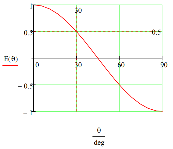
Demonstrate that a hidden-value model that agrees with the 0 and 90 degree quantum expectation values, disagrees with the 30 degree result.

Hidden variable expectation value for 30 degrees:

\[
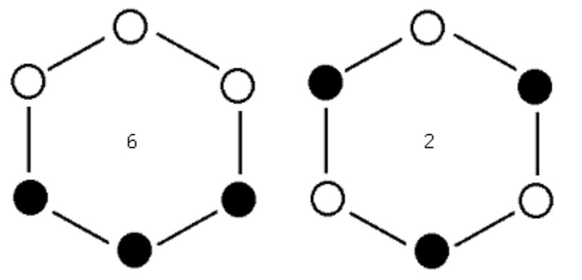
\frac{6 \cdot(1-1+1+1-1+1)+2 \cdot(-1-1-1-1-1-1)}{8}=0
\nonumber \]

I turn to David Lindley again (Where Does the Weirdness Go? page 15) for a concluding comment on the issues dealt with in this section.

We are, through long familiarity, grounded in the assumption of an external, objective, and definite reality, regardless of how much or how little we actually know about it. It is hard to find the language or the concepts to deal with a “reality” that only becomes real when it is measured. There is no easy way to grasp this change of perspective, but persistence and patience allow a certain new familiarity to supplant the old.

Bibliography

• The Quest for the Quantum Computer, Julian Brown
• The Meaning of Quantum Theory, Jim Baggott
• Quantum Reality, Nick Herbert
• Where Does the Weirdness Go?, David Lindley
• The Cosmic Code, Heinz Pagels
• Quantum Mechanics and Experience, David Z Albert
• Quantum Mechanics, Alastair Rae
• Quantum Physics: Illusion or Reality, Alastair Rae
• The Quantum Divide, Gerry and Bruno
• Quantum Weirdness, William J. Mullin
• Through Two Doors at Once, Anil Ananthaswamy
• Beyond Weird, Philip Ball
• Quantum Physics: What Everyone Needs to Know, Michael G. Raymer
• Quantum Theory: A Very Short Introduction, John Polkinhorne
• The Quantum Challenge, Greenstein and Zajonc
• Quantum Enigma, Rosenblum and Kuttner
• Programming the Universe, Seth Lloyd