1.7: Quantum Computation- A Short Course
- Page ID
- 136092

\( \newcommand{\vecs}[1]{\overset { \scriptstyle \rightharpoonup} {\mathbf{#1}} } \)
\( \newcommand{\vecd}[1]{\overset{-\!-\!\rightharpoonup}{\vphantom{a}\smash {#1}}} \)
\( \newcommand{\id}{\mathrm{id}}\) \( \newcommand{\Span}{\mathrm{span}}\)
( \newcommand{\kernel}{\mathrm{null}\,}\) \( \newcommand{\range}{\mathrm{range}\,}\)
\( \newcommand{\RealPart}{\mathrm{Re}}\) \( \newcommand{\ImaginaryPart}{\mathrm{Im}}\)
\( \newcommand{\Argument}{\mathrm{Arg}}\) \( \newcommand{\norm}[1]{\| #1 \|}\)
\( \newcommand{\inner}[2]{\langle #1, #2 \rangle}\)
\( \newcommand{\Span}{\mathrm{span}}\)
\( \newcommand{\id}{\mathrm{id}}\)
\( \newcommand{\Span}{\mathrm{span}}\)
\( \newcommand{\kernel}{\mathrm{null}\,}\)
\( \newcommand{\range}{\mathrm{range}\,}\)
\( \newcommand{\RealPart}{\mathrm{Re}}\)
\( \newcommand{\ImaginaryPart}{\mathrm{Im}}\)
\( \newcommand{\Argument}{\mathrm{Arg}}\)
\( \newcommand{\norm}[1]{\| #1 \|}\)
\( \newcommand{\inner}[2]{\langle #1, #2 \rangle}\)
\( \newcommand{\Span}{\mathrm{span}}\) \( \newcommand{\AA}{\unicode[.8,0]{x212B}}\)
\( \newcommand{\vectorA}[1]{\vec{#1}} % arrow\)
\( \newcommand{\vectorAt}[1]{\vec{\text{#1}}} % arrow\)
\( \newcommand{\vectorB}[1]{\overset { \scriptstyle \rightharpoonup} {\mathbf{#1}} } \)
\( \newcommand{\vectorC}[1]{\textbf{#1}} \)
\( \newcommand{\vectorD}[1]{\overrightarrow{#1}} \)
\( \newcommand{\vectorDt}[1]{\overrightarrow{\text{#1}}} \)
\( \newcommand{\vectE}[1]{\overset{-\!-\!\rightharpoonup}{\vphantom{a}\smash{\mathbf {#1}}}} \)
\( \newcommand{\vecs}[1]{\overset { \scriptstyle \rightharpoonup} {\mathbf{#1}} } \)
\( \newcommand{\vecd}[1]{\overset{-\!-\!\rightharpoonup}{\vphantom{a}\smash {#1}}} \)
\(\newcommand{\avec}{\mathbf a}\) \(\newcommand{\bvec}{\mathbf b}\) \(\newcommand{\cvec}{\mathbf c}\) \(\newcommand{\dvec}{\mathbf d}\) \(\newcommand{\dtil}{\widetilde{\mathbf d}}\) \(\newcommand{\evec}{\mathbf e}\) \(\newcommand{\fvec}{\mathbf f}\) \(\newcommand{\nvec}{\mathbf n}\) \(\newcommand{\pvec}{\mathbf p}\) \(\newcommand{\qvec}{\mathbf q}\) \(\newcommand{\svec}{\mathbf s}\) \(\newcommand{\tvec}{\mathbf t}\) \(\newcommand{\uvec}{\mathbf u}\) \(\newcommand{\vvec}{\mathbf v}\) \(\newcommand{\wvec}{\mathbf w}\) \(\newcommand{\xvec}{\mathbf x}\) \(\newcommand{\yvec}{\mathbf y}\) \(\newcommand{\zvec}{\mathbf z}\) \(\newcommand{\rvec}{\mathbf r}\) \(\newcommand{\mvec}{\mathbf m}\) \(\newcommand{\zerovec}{\mathbf 0}\) \(\newcommand{\onevec}{\mathbf 1}\) \(\newcommand{\real}{\mathbb R}\) \(\newcommand{\twovec}[2]{\left[\begin{array}{r}#1 \\ #2 \end{array}\right]}\) \(\newcommand{\ctwovec}[2]{\left[\begin{array}{c}#1 \\ #2 \end{array}\right]}\) \(\newcommand{\threevec}[3]{\left[\begin{array}{r}#1 \\ #2 \\ #3 \end{array}\right]}\) \(\newcommand{\cthreevec}[3]{\left[\begin{array}{c}#1 \\ #2 \\ #3 \end{array}\right]}\) \(\newcommand{\fourvec}[4]{\left[\begin{array}{r}#1 \\ #2 \\ #3 \\ #4 \end{array}\right]}\) \(\newcommand{\cfourvec}[4]{\left[\begin{array}{c}#1 \\ #2 \\ #3 \\ #4 \end{array}\right]}\) \(\newcommand{\fivevec}[5]{\left[\begin{array}{r}#1 \\ #2 \\ #3 \\ #4 \\ #5 \\ \end{array}\right]}\) \(\newcommand{\cfivevec}[5]{\left[\begin{array}{c}#1 \\ #2 \\ #3 \\ #4 \\ #5 \\ \end{array}\right]}\) \(\newcommand{\mattwo}[4]{\left[\begin{array}{rr}#1 \amp #2 \\ #3 \amp #4 \\ \end{array}\right]}\) \(\newcommand{\laspan}[1]{\text{Span}\{#1\}}\) \(\newcommand{\bcal}{\cal B}\) \(\newcommand{\ccal}{\cal C}\) \(\newcommand{\scal}{\cal S}\) \(\newcommand{\wcal}{\cal W}\) \(\newcommand{\ecal}{\cal E}\) \(\newcommand{\coords}[2]{\left\{#1\right\}_{#2}}\) \(\newcommand{\gray}[1]{\color{gray}{#1}}\) \(\newcommand{\lgray}[1]{\color{lightgray}{#1}}\) \(\newcommand{\rank}{\operatorname{rank}}\) \(\newcommand{\row}{\text{Row}}\) \(\newcommand{\col}{\text{Col}}\) \(\renewcommand{\row}{\text{Row}}\) \(\newcommand{\nul}{\text{Nul}}\) \(\newcommand{\var}{\text{Var}}\) \(\newcommand{\corr}{\text{corr}}\) \(\newcommand{\len}[1]{\left|#1\right|}\) \(\newcommand{\bbar}{\overline{\bvec}}\) \(\newcommand{\bhat}{\widehat{\bvec}}\) \(\newcommand{\bperp}{\bvec^\perp}\) \(\newcommand{\xhat}{\widehat{\xvec}}\) \(\newcommand{\vhat}{\widehat{\vvec}}\) \(\newcommand{\uhat}{\widehat{\uvec}}\) \(\newcommand{\what}{\widehat{\wvec}}\) \(\newcommand{\Sighat}{\widehat{\Sigma}}\) \(\newcommand{\lt}{<}\) \(\newcommand{\gt}{>}\) \(\newcommand{\amp}{&}\) \(\definecolor{fillinmathshade}{gray}{0.9}\)As can be seen in the previous tutorials, teleportation involves entanglement transfer. Alice projects her photons onto one of the entangled Bell states and Bob receives a photon state which using information provided via the classical communication channel can be transformed into the teleportee state. Given the importance of entanglement in quantum computing a more elaborate example of entanglement transfer is provided in the following tutorial.
An Entanglement Swapping Protocol
In the field of quantum information interference, superpositions and entangled states are essential resources. Entanglement, a non-factorable superposition, is routinely achieved when two photons are emitted from the same source, say a parametric down converter (PDC). Entanglement swapping involves the transfer of entanglement to two photons that were produced independently and never previously interacted. The Bell states are the four maximally entangled two-qubit entangled basis for a four-dimensional Hilbert space and play an essential role in quantum information theory and technology, including teleportation and entanglement swapping. The Bell states are shown below.
\[\begin{array} a \Phi_{\mathrm{p}}=\dfrac{1}{\sqrt{2}} \cdot\left[\left( \begin{array}{l}{1} \\ {0}\end{array}\right) \cdot \left( \begin{array}{l}{1} \\ {0}\end{array}\right)+\left( \begin{array}{l}{0} \\ {1}\end{array}\right) \cdot \left( \begin{array}{l}{0} \\ {1}\end{array}\right)\right] \quad & \Phi_{\mathrm{p}} :=\dfrac{1}{\sqrt{2}} \cdot \left( \begin{array}{l}{1} \\ {0} \\ {0} \\ {1}\end{array}\right) \quad & \Phi_{\mathrm{m}}=\dfrac{1}{\sqrt{2}} \cdot\left[\left( \begin{array}{l}{1} \\ {0}\end{array}\right) \cdot \left( \begin{array}{l}{1} \\ {0}\end{array}\right)-\left( \begin{array}{l}{0} \\ {1}\end{array}\right) \cdot \left( \begin{array}{l}{0} \\ {1}\end{array}\right)\right] \quad & \Phi_{\mathrm{m}} :=\dfrac{1}{\sqrt{2}} \cdot \left( \begin{array}{c}{1} \\ {0} \\ {0} \\ {-1}\end{array}\right) \\ \Psi_{\mathrm{p}}=\dfrac{1}{\sqrt{2}} \cdot\left[\left( \begin{array}{l}{1} \\ {0}\end{array}\right) \cdot \left( \begin{array}{l}{0} \\ {1}\end{array}\right)+\left( \begin{array}{l}{1} \\ {0}\end{array}\right) \cdot \left( \begin{array}{l}{0} \\ {1}\end{array}\right)\right] \quad & \Psi_{\mathrm{p}} :=\dfrac{1}{\sqrt{2}} \cdot \left( \begin{array}{l}{0} \\ {1} \\ {1} \\ {0}\end{array}\right) & \Psi_{\mathrm{m}}=\dfrac{1}{\sqrt{2}} \cdot\left[\left( \begin{array}{l}{1} \\ {0}\end{array}\right) \cdot \left( \begin{array}{l}{0} \\ {1}\end{array}\right)-\left( \begin{array}{l}{0} \\ {1}\end{array}\right) \cdot \left( \begin{array}{l}{1} \\ {0}\end{array}\right)\right] \quad & \Psi_{\mathrm{m}} :=\dfrac{1}{\sqrt{2}} \left( \begin{array}{c}{0} \\ {1} \\ {-1} \\ {0}\end{array}\right) \end{array} \nonumber \]
A four-qubit state is prepared in which photons 1 and 2 are entangled in Bell state \(\Phi_{p}\), and photons 3 and 4 are entangled in Bell state \(\Psi_{m}\). The state multiplication below is understood to be tensor vector multiplication.
\[
\Psi=\Phi_{\mathrm{p}} \cdot \Psi_{\mathrm{m}}=\frac{1}{\sqrt{2}} \cdot \left( \begin{array}{l}{1} \\ {0} \\ {0} \\ {1}\end{array}\right) \cdot \frac{1}{\sqrt{2}} \cdot \left( \begin{array}{c}{0} \\ {1} \\ {-1} \\ {0}\end{array}\right) \quad \Psi :=\frac{1}{2} \cdot \left( \begin{array}{ccccccccccccccc}{0} & {1} & {-1} & {0} & {0} & {0} & {0} & {0} & {0} & {0} & {0} & {0} & {0} & {1} & {-1} & {0}\end{array}\right)^{\mathrm{T}} \quad \mathrm{I} :=\left( \begin{array}{ll}{1} & {0} \\ {0} & {1}\end{array}\right)
\nonumber \]
Four Bell state measurements are now made on photons 2 and 3 which entangles photons 1 and 4. Projection of photons 2 and 3 onto \(\Phi_{p}\) projects photons 1 and 4 onto \(\Psi_{m}\).
\[
\left(\text { kronecker }\left(\mathrm{I}, \text { kronecker }\left(\Phi_{\mathrm{p}} \cdot \Phi_{\mathrm{p}}^{\mathrm{T}}, \mathrm{I}\right)\right) \cdot \Psi\right)^{\mathrm{T}}=\left( \begin{array}{llllllllllllll}{0} & {0.25} & {0} & {0} & {0} & {0} & {0} & {0.25} & {-0.25} & {0} & {0} & {0} & {0} & {0} & {-0.25} & {0}\end{array}\right)
\nonumber \]
\[
\frac{1}{2 \sqrt{2}} \cdot\left[\left( \begin{array}{c}{1} \\ {0}\end{array}\right) \cdot \frac{1}{\sqrt{2}} \cdot \left( \begin{array}{l}{1} \\ {0} \\ {0} \\ {1}\end{array}\right) \cdot \left( \begin{array}{l}{0} \\ {1}\end{array}\right) -\left( \begin{array}{l}{0} \\ {1}\end{array}\right) \cdot \frac{1}{\sqrt{2}}\cdot\left( \begin{array}{l}{1} \\ {0} \\ {0} \\ {1}\end{array}\right) \cdot \left( \begin{array}{l}{1} \\ {0}\end{array}\right)\right]^{T} \\ =\frac{1}{4} \cdot \left( \begin{array}{llllllllllll}{0} & {1} & {0} & {0} & {0} & {0} & {0 }& {1} & {-1} & {0} & {0} & {0} & {0} & {0} & {-1} & {0}\end{array}\right)
\nonumber \]
Projection of photons 2 and 3 onto \(\Phi_{m}\) projects photons 1 and 4 onto \(\Psi_{p}\).
\[
\left(\text { kronecker }\left(\mathrm{I}, \text { kronecker }\left(\Phi_{\mathrm{m}} \cdot \Phi_{\mathrm{m}}^{\mathrm{T}}, \mathrm{I}\right)\right) \cdot \Psi\right)^{\mathrm{T}}=\left( \begin{array}{llllllllllllll}{0} & {0.25} & {0} & {0} & {0} & {0} & {0} & {-0.25} & {0.25} & {0} & {0} & {0} & {0} & {0} & {-0.25} & {0}\end{array}\right)
\nonumber \]
\[
\frac{1}{2 \sqrt{2}} \cdot\left[\left( \begin{array}{c}{1} \\ {0}\end{array}\right) \cdot \frac{1}{\sqrt{2}} \cdot \left( \begin{array}{l}{1} \\ {0} \\ {0} \\ {-1}\end{array}\right) \cdot \left( \begin{array}{l}{0} \\ {1}\end{array}\right) +\left( \begin{array}{l}{0} \\ {1}\end{array}\right) \cdot \frac{1}{\sqrt{2}}\cdot\left( \begin{array}{l}{1} \\ {0} \\ {0} \\ {-1}\end{array}\right) \cdot \left( \begin{array}{l}{1} \\ {0}\end{array}\right)\right]^{T} \\ =\frac{1}{4} \cdot \left( \begin{array}{llllllllllll}{0} & {1} & {0} & {0} & {0} & {0} & {0 }& {-1} & {1} & {0} & {0} & {0} & {0} & {0} & {-1} & {0}\end{array}\right)
\nonumber \]
Projection of photons 2 and 3 onto \(\Psi_{p}\) projects photons 1 and 4 onto \(\Phi_{m}\).
\[
\left(\text { kronecker }\left(\mathrm{I}, \text { kronecker }\left(\Phi_{\mathrm{p}} \cdot \Phi_{\mathrm{p}}^{\mathrm{T}}, \mathrm{I}\right)\right) \cdot \Psi\right)^{\mathrm{T}}=\left( \begin{array}{llllllllllllll}{0} & {0} & {-0.25} & {0} & {-0.25} & {0} & {0} & {0} & {0} & {0} & {0} & {0.25} & {0} & {0.25} & {0} & {0}\end{array}\right)
\nonumber \]
\[
\frac{1}{2 \sqrt{2}} \cdot\left[\left( \begin{array}{c}{0} \\ {1}\end{array}\right) \cdot \frac{1}{\sqrt{2}} \cdot \left( \begin{array}{l}{0} \\ {1} \\ {1} \\ {0}\end{array}\right) \cdot \left( \begin{array}{l}{0} \\ {1}\end{array}\right) -\left( \begin{array}{l}{1} \\ {0}\end{array}\right) \cdot \frac{1}{\sqrt{2}}\cdot\left( \begin{array}{l}{0} \\ {1} \\ {1} \\ {0}\end{array}\right) \cdot \left( \begin{array}{l}{1} \\ {0}\end{array}\right)\right]^{T} \\ =\frac{1}{4} \cdot \left( \begin{array}{llllllllllll}{0} & {0} & {-1} & {0} & {-1} & {0} & {0}& {0} & {0} & {0} & {0} & {1} & {0} & {1} & {0} & {0}\end{array}\right)
\nonumber \]
Finally, projection of photons 2 and 3 onto \(\Phi_{m}\) projects photons 1 and 4 onto \(\Psi_{p}\).
\[
\left(\text { kronecker }\left(\mathrm{I}, \text { kronecker }\left(\Phi_{\mathrm{m}} \cdot \Phi_{\mathrm{m}}^{\mathrm{T}}, \mathrm{I}\right)\right) \cdot \Psi\right)^{\mathrm{T}}=\left( \begin{array}{llllllllllllll}{0} & {0} & {-0.25} & {0} & {0.25} & {0} & {0} & {0} & {0} & {0} & {0} & {-0.25} & {0} & {0.25} & {0} & {0}\end{array}\right)
\nonumber \]
\[
\frac{-1}{2 \sqrt{2}} \cdot\left[\left( \begin{array}{c}{1} \\ {0}\end{array}\right) \cdot \frac{1}{\sqrt{2}} \cdot \left( \begin{array}{l}{0} \\ {1} \\ {-1} \\ {0}\end{array}\right) \cdot \left( \begin{array}{l}{1} \\ {0}\end{array}\right) +\left( \begin{array}{l}{0} \\ {1}\end{array}\right) \cdot \frac{1}{\sqrt{2}}\cdot\left( \begin{array}{l}{0} \\ {1} \\ {-1} \\ {0}\end{array}\right) \cdot \left( \begin{array}{l}{0} \\ {1}\end{array}\right)\right]^{T} \\ =\frac{1}{4} \cdot \left( \begin{array}{llllllllllll}{0} & {0} & {-1} & {0} & {1} & {0} & {0}& {0} & {0} & {0} & {0} & {-1} & {0} & {1} & {0} & {0}\end{array}\right)
\nonumber \]
In our earlier examination of the quantum computer we saw that a quantum circuit can calculate all the values of f(x) simultaneously, but we can only retrieve one value due to the collapse of the superposition of answers on observation. To achieve a quantum advantage in computation requires more subtle programming techniques which exploit the effects of quantum interference. The following tutorials reveal how the quantum advantage can be achieved in several areas of practical importance.
While quantum mechanics could spell disaster for public-key cryptography, it may also offer salvation. This is because the resources of the quantum world appear to offer the ultimate form of secret code, one that is guaranteed by the laws of physics to be unbreakable. Julian Brown, The Quest for the Quantum Computer, page 189.
In other words, “The quantum taketh away and the quantum giveth back!” Asher Peres
We begin with Shor’s algorithm which demonstrates how quantum entanglement and interference effects can facilitate the factorization of large integers into their prime factors. The inability of conventional computers to do this is essential to the integrity of public-key cryptography.
Factoring Using Shor's Quantum Algorithm
This tutorial presents a toy calculation dealing with quantum factorization using Shor's algorithm. Before beginning that task, traditional classical factorization is reviewed with the example of finding the prime factors of 15. As shown below the key is to find the period of ax modulo 15, where a is chosen randomly.
\[
\mathrm{a} :=4 \qquad \mathrm{N} :=15 \qquad f(x) :=\bmod \left(a^{x}, N\right) \qquad \mathrm{Q} :=8 \qquad \mathrm{x} :=0 \ldots \mathrm{Q}-1
\nonumber \]
| x | f(x) |
|---|---|
| 0 | 1 |
| 1 | 4 |
| 2 | 1 |
| 3 | 4 |
| 4 | 1 |
| 5 | 4 |
| 6 | 1 |
| 7 | 4 |
Seeing that the period of f(x) is two, the next step is to use the Euclidian algorithm by calculating the greatest common denominator of two functions involving the period and a, and the number to be factored, N.
\[ \text{period} : = 2 \qquad \operatorname{gcd}\left(a^{\frac{\text { period }}{2}}-1, \mathrm{N}\right)=3 \qquad \operatorname{gcd}\left(a^{\frac{\text { period }}{2}}+1, \mathrm{N}\right)=5 \nonumber \]
We proceed by ignoring the fact that we already know that the period of f(x) is 2 and demonstrate how it is determined using a quantum (discrete) Fourier transform. After the registers are loaded with x and f(x) using a quantum computer, they exist in the following superposition.
\[
\frac{1}{\sqrt{Q}} \sum_{x=0}^{Q-1} | x \rangle | f(x) \rangle=\frac{1}{2}[ |0\rangle | 1 \rangle+| 1 \rangle | 4 \rangle+| 2 \rangle | 1 \rangle+| 3 \rangle | 4 \rangle+\cdots ]
\nonumber \]
The next step is to find the period of f(x) by performing a quantum Fourier transform (QFT) on the input register |x>.
\[
\mathrm{Q} :=4 \qquad \mathrm{m} :=0 \ldots \mathrm{Q}-1 \qquad \mathrm{n} :=0 . \mathrm{Q}-1 \qquad \mathrm{QFT}_{\mathrm{m}, \mathrm{n}} :=\frac{1}{\sqrt{\mathrm{Q}}} \cdot \exp \left(\mathrm{i} \cdot \frac{2 \cdot \pi \cdot \mathrm{m} \cdot \mathrm{n}}{\mathrm{Q}}\right) \qquad \mathrm{QFT}=\frac{1}{2} \cdot \left( \begin{array}{cccc}{1} & {1} & {1} & {1} \\ {1} & {\mathrm{i}} & {-1} & {-\mathrm{i}} \\ {1} & {-1} & {1} & {-1} \\ {1} & {-\mathrm{i}} & {-1} & {\mathrm{i}}\end{array}\right)
\nonumber \]
\[
\mathrm{x}=0 \quad \mathrm{QFT} \cdot \left( \begin{array}{l}{1} \\ {0} \\ {0} \\ {0}\end{array}\right)=\left( \begin{array}{c}{0.5} \\ {0.5} \\ {0.5} \\ {0.5}\end{array}\right) \qquad \mathrm{x}=1 \quad \mathrm{QFT} \cdot \left( \begin{array}{l}{0} \\ {1} \\ {0} \\ {0}\end{array}\right)=\left( \begin{array}{c}{0.5} \\ {0.5 \mathrm{i}} \\ {-0.5} \\ {-0.5 \mathrm{i}}\end{array}\right) \\ \mathrm{x}=2 \quad \mathrm{QFT} \cdot \left( \begin{array}{l}{0} \\ {0} \\ {1} \\ {0}\end{array}\right)=\left( \begin{array}{c}{0.5} \\ {-0.5} \\ {0.5} \\ {-0.5}\end{array}\right) \qquad \mathrm{x}=3 \quad \mathrm{QFT} \cdot \left( \begin{array}{l}{0} \\ {0} \\ {0} \\ {1}\end{array}\right)=\left( \begin{array}{c}{0.5} \\ {-0.5 \mathrm{i}} \\ {-0.5} \\ {0.5 \mathrm{i}}\end{array}\right)
\nonumber \]
The operation of the QFT on the x-register is expressed algebraically in the middle term below. Quantum interference in this term yields the result on the right which shows a period of 2 on the x-register.
\[\begin{array} a \; & \frac{1}{4}[ |0\rangle+| 1 \rangle+| 2 \rangle+| 3 \rangle ] | 1 \rangle & \\ \; & \qquad \qquad \quad + & \; \\ \; & \frac{1}{4}[ |0\rangle+ i | 1 \rangle-| 2 \rangle-i | 3 \rangle ] | 4 \rangle & \; \\ Q F T(x) \frac{1}{2}[ |0\rangle | 1 \rangle+| 1 \rangle | 4 \rangle+| 2 \rangle | 1 \rangle+| 3 \rangle | 4 \rangle ]= & \qquad \qquad \quad + & =\frac{1}{2}[ |0\rangle( |1\rangle+| 4 \rangle )+| 2 \rangle( |1\rangle-| 4 \rangle ) ] \\ \; & \frac{1}{4}[ |0\rangle-| 1 \rangle+| 2 \rangle-| 3 \rangle ] | 1 \rangle & \; \\ \; & \qquad \qquad \quad + & \; \\ \; & \frac{1}{4}[ |0\rangle- i | 1 \rangle-| 2 \rangle+i | 3 \rangle ] | 4 \rangle & \; \end{array} \nonumber \]
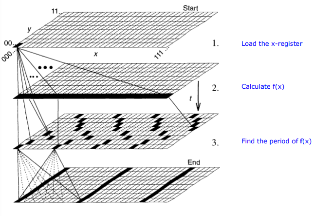
Figure 5 in "Quantum Computation," by David P. DiVincenzo, Science 270, 258 (1995) provides a graphical illustration of the steps of Shor's factorization algorithm.
How quantum theory gives back is demonstrated by an examination of Ekert’s quantum secret key proposal.
The Quantum Math Behind Ekert's Key Distribution Scheme
Alice and Bob share an entangled photon (EPR) pair in the following state.
\[
\begin{split} | \Psi \rangle &=\frac{1}{\sqrt{2}}[ |\mathrm{R}\rangle_{A} | \mathrm{R} \rangle_{\mathrm{B}}+| \mathrm{L} \rangle_{\mathrm{A}} | \mathrm{L} \rangle_{\mathrm{B}} ] =\frac{1}{2 \sqrt{2}}\left[\left( \begin{array}{c}{1} \\ {i}\end{array}\right)_{A} \otimes \left( \begin{array}{l}{1} \\ {i}\end{array}\right)_{B}+\left( \begin{array}{c}{1} \\ {-i}\end{array}\right)_{A} \otimes \left( \begin{array}{c}{1} \\ {-i}\end{array}\right)_{B}\right] \\ &=\frac{1}{\sqrt{2}} \left( \begin{array}{c}{1} \\ {0} \\ {0} \\ {-1}\end{array}\right)=\frac{1}{\sqrt{2}}[ |\mathrm{V}\rangle_{\mathrm{A}} | \mathrm{V} \rangle_{\mathrm{B}}-| \mathrm{H} \rangle_{\mathrm{A}} | \mathrm{H} \rangle_{\mathrm{B}} ] \end{split}
\nonumber \]
They agree to make random polarization measurements in the rectilinear and circular polarization bases. When a measurement is made on a quantum system the result is always an eigenstate of the measurement operator. The eigenstates in the circular and rectilinear bases are:
\[
\mathrm{R} :=\frac{1}{\sqrt{2}} \cdot \left( \begin{array}{l}{1} \\ {\mathrm{i}}\end{array}\right) \quad \mathrm{L} :=\frac{1}{\sqrt{2}} \cdot \left( \begin{array}{c}{1} \\ {-\mathrm{i}}\end{array}\right) \quad \mathrm{V} :=\left( \begin{array}{l}{1} \\ {0}\end{array}\right) \quad \mathrm{H} :=\left( \begin{array}{l}{0} \\ {1}\end{array}\right)
\nonumber \]
Pertinent superpositions:
\[
\mathrm{V}=\frac{1}{\sqrt{2}} \cdot(\mathrm{R}+\mathrm{L}) \quad \mathrm{H}=\frac{\mathrm{i}}{\sqrt{2}} \cdot(\mathrm{L}-\mathrm{R}) \quad \mathrm{R}=\frac{1}{\sqrt{2}} \cdot(\mathrm{V}+\mathrm{i} \cdot \mathrm{H}) \quad \mathrm{L}=\frac{1}{\sqrt{2}} \cdot(\mathrm{V}-\mathrm{i} \cdot \mathrm{H})
\nonumber \]
Alice's random measurement effectively sends a random photon to Bob due to the correlations built into the entangled state of their shared photon pair. Alice's four measurement possibilities and their consequences for Bob are now examined.
Alice's photon is found to be right circularly polarized, |R>. If Bob measures circular polarization he is certain to find his photon to be |R>. But if he chooses to measure in the rectilinear basis the probability he will observe |V> is 0.5 and the probability he will observe |H> is 0.5.
\[
\frac{1}{\sqrt{2}} \cdot \mathrm{R} \cdot \mathrm{R}=\frac{1}{\sqrt{2}} \cdot \mathrm{R} \cdot\left[\frac{1}{\sqrt{2}} \cdot(\mathrm{V}+\mathrm{i} \cdot \mathrm{H})\right]
\nonumber \]
If Alice observes |L>, Bob will also if he measures circular polarization. But if he measures in the rectilinear basis the probability he will observe |V> is 0.5 and the probability he will observe |H> is 0.5.
\[
\frac{1}{\sqrt{2}} \cdot \mathrm{L} \cdot \mathrm{L}=\frac{1}{\sqrt{2}} \cdot \mathrm{L} \cdot\left[\frac{1}{\sqrt{2}} \cdot(\mathrm{V}-\mathrm{i} \cdot \mathrm{H})\right]
\nonumber \]
The same kind of reasoning applies to measurements Alice makes in the rectilinear basis.
\[
\frac{1}{\sqrt{2}} \cdot \mathrm{V} \cdot \mathrm{V}=\frac{1}{\sqrt{2}} \cdot \mathrm{V} \cdot\left[\frac{1}{\sqrt{2}} \cdot(\mathrm{R}+\mathrm{L})\right] \qquad \frac{1}{\sqrt{2}} \cdot \mathrm{H} \cdot \mathrm{H}=-\frac{1}{\sqrt{2}} \cdot \mathrm{H} \cdot\left[\frac{\mathrm{i}}{\sqrt{2}} \cdot(\mathrm{L}-\mathrm{R})\right]
\nonumber \]
Alice and Bob keep the results for the experiments for which they measured in the same basis (blue in the table below), and make the following bit value assignments: |V> = |R> = 0 and |H> = |L> = 1. This leads to the secret key on the bottom line.
\[
\begin{array}{llllllllll}{\text {Alice }} & {\mathrm{R}} & {\mathrm{V}} & {\mathrm{V}} & {\mathrm{L}} & {\mathrm{H}} & {\mathrm{L}} & {\mathrm{H}} & {\mathrm{R}} & {\mathrm{V}} & {\mathrm{L}} & {\mathrm{H}} \\ {\mathrm{Bob}} & {\mathrm{R}} & {\mathrm{L}} & {\mathrm{V}} & {\mathrm{L}} & {\mathrm{R}} & {\mathrm{H}} & {\mathrm{H}} & {\mathrm{R}} & {\mathrm{V}} & {\mathrm{V}} & {\mathrm{H}} \\ {\mathrm{Key}} & {0} & \; &{0} & {1} & \; & \; & {1} & {0} & {0} & \; & {1}\end{array}
\nonumber \]
The following demonstrates how a binary message is coded and subsequently decoded using a shared binary secret key and modulo 2 arithmetic.
| Message | Key | Coded Message | Decoded Message |
|---|---|---|---|
| $$ \text{Mes} : = \begin{pmatrix} 0 \\ 1 \\ 0 \\ 0 \\ 0 \\ 1 \\ 1 \\ 0 \\ 0 \\ 1 \\ 0 \\ 1 \\ 0 \\ 1 \end{pmatrix} $$ |
$$ \text{Key} : = \begin{pmatrix} 0 \\ 0 \\ 1 \\ 1 \\ 0 \\ 0 \\ 1 \\ 0 \\ 0 \\ 1 \\ 1 \\ 0 \\ 0 \\ 1 \end{pmatrix} $$ |
$$ \mathrm{CMes} :=\bmod (\mathrm{Mes}+\mathrm{Key}, 2)\begin{pmatrix} 0 \\ 1 \\ 1 \\ 1 \\ 0 \\ 1 \\ 0 \\ 0 \\ 0 \\ 0 \\ 1 \\ 1 \\ 0 \\ 1 \end{pmatrix} $$ |
$$ \mathrm{DMes} :=\bmod (\mathrm{CMes}+\mathrm{Key}, 2)\begin{pmatrix} 0 \\ 1 \\ 0 \\ 0 \\ 0 \\ 1 \\ 1 \\ 0 \\ 0 \\ 1 \\ 0 \\ 1 \\ 0 \\ 1 \end{pmatrix} $$ |
It is clear by inspection that the message has been accurately decoded. This is confirmed by calculating the difference between the message and the decoded message.
\[
(\mathrm{Mes}-\mathrm{DMes})^{\mathrm{T}}=\left( \begin{array}{lllllllllllll}{0} & {0} & {0} & {0} & {0} & {0} & {0} & {0} & {0} & {0} & {0} & {0} & {0} & {0}\end{array}\right)
\nonumber \]
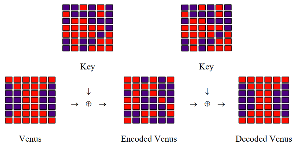
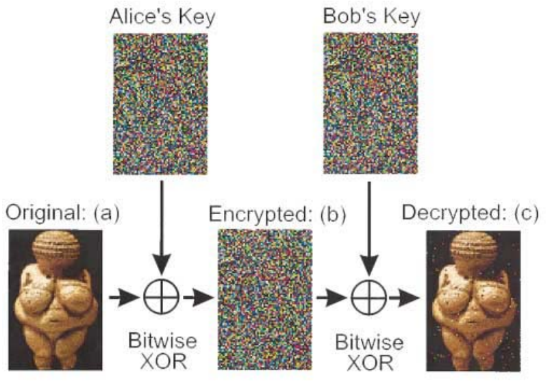
Coding and Decoding Venus
In 2000 Anton Zeilinger and his research team sent an encrypted photo of the fertility goddess Venus of Willendorf from Alice to Bob, two computers in two buildings about 400 meters apart. The figure summarizing this achievement first appeared in Physical Review Letters and later in a review article in Nature.
It is easy to produce a rudimentary simulation of the experiment. Bitwise XOR is nothing more than addition modulo 2. The original Venus and the shared key are represented by the following matrices, where the matrix elements are pixels that are either off (0) or on (1).
\[
\mathrm{i}=1 . .7 \qquad \mathrm{j} :=1 . .6 \qquad \mathrm{Key}_{\mathrm{i}, \mathrm{j}} :=\operatorname{trunc}(\mathrm{md}(2))
\nonumber \]
\[
\text{Key }=\left( \begin{array}{cccccc}{0} & {0} & {1} & {0} & {1} & {0} \\ {1} & {0} & {0} & {0} & {1} & {0} \\ {0} & {1} & {1} & {0} & {0} & {0} \\ {1} & {1} & {1} & {1} & {1} & {0} \\ {1} & {1} & {1} & {1} & {0} & {1} \\ {0} & {1} & {0} & {0} & {1} & {1} \\ {0} & {1} & {0} & {1} & {1} & {1}\end{array}\right)
\nonumber \]
\[
\text{Venus }: =\left( \begin{array}{cccccc}{1} & {1} & {1} & {1} & {1} & {1} \\ {0} & {1} & {1} & {1} & {1} & {0} \\ {0} & {0} & {1} & {1} & {0} & {0} \\ {0} & {0} & {1} & {1} & {0} & {0} \\ {0} & {0} & {1} & {1} & {0} & {0} \\ {0} & {1} & {1} & {1} & {1} & {0} \\ {1} & {1} & {1} & {1} & {1} & {1}\end{array}\right)
\nonumber \]
A coded version of Venus is prepared by adding Venus and the Key modulo 2 and sent to Bob.
\[
C_{i, j} :=\text { Venus }_{i, j} \oplus K e y_{i, j} \qquad \text{CVenus}=\left( \begin{array}{cccccc}{1} & {1} & {0} & {1} & {0} & {1} \\ {1} & {1} & {1} & {1} & {0} & {0} \\ {0} & {1} & {0} & {1} & {0} & {0} \\ {1} & {1} & {0} & {0} & {1} & {0} \\ {1} & {1} & {0} & {0} & {0} & {1} \\ {0} & {0} & {1} & {1} & {0} & {1} \\ {1} & {0} & {1} & {0} & {0} & {0}\end{array}\right)
\nonumber \]
Bob adds the key to CVenus modulo 2 and sends the result to his printer.
\[
\mathrm{DVenus}_{\mathrm{i}, \mathrm{j}} :=\mathrm{CVenus}_{\mathrm{i}, \mathrm{j}} \oplus \mathrm{Key}_{\mathrm{i}, \mathrm{j}} \qquad
\text{DVenus}=\left( \begin{array}{cccccc}{1} & {1} & {1} & {1} & {1} & {1} \\ {0} & {1} & {1} & {1} & {1} & {0} \\ {0} & {0} & {1} & {1} & {0} & {0} \\ {0} & {0} & {1} & {1} & {0} & {0} \\ {0} & {0} & {1} & {1} & {0} & {0} \\ {0} & {1} & {1} & {1} & {1} & {0} \\ {1} & {1} & {1} & {1} & {1} & {1}\end{array}\right)
\nonumber \]
A graphic summary of the simulation: