
Potential Energy Surface
- Page ID
- 73970
\( \newcommand{\vecs}[1]{\overset { \scriptstyle \rightharpoonup} {\mathbf{#1}} } \)
\( \newcommand{\vecd}[1]{\overset{-\!-\!\rightharpoonup}{\vphantom{a}\smash {#1}}} \)
\( \newcommand{\dsum}{\displaystyle\sum\limits} \)
\( \newcommand{\dint}{\displaystyle\int\limits} \)
\( \newcommand{\dlim}{\displaystyle\lim\limits} \)
\( \newcommand{\id}{\mathrm{id}}\) \( \newcommand{\Span}{\mathrm{span}}\)
( \newcommand{\kernel}{\mathrm{null}\,}\) \( \newcommand{\range}{\mathrm{range}\,}\)
\( \newcommand{\RealPart}{\mathrm{Re}}\) \( \newcommand{\ImaginaryPart}{\mathrm{Im}}\)
\( \newcommand{\Argument}{\mathrm{Arg}}\) \( \newcommand{\norm}[1]{\| #1 \|}\)
\( \newcommand{\inner}[2]{\langle #1, #2 \rangle}\)
\( \newcommand{\Span}{\mathrm{span}}\)
\( \newcommand{\id}{\mathrm{id}}\)
\( \newcommand{\Span}{\mathrm{span}}\)
\( \newcommand{\kernel}{\mathrm{null}\,}\)
\( \newcommand{\range}{\mathrm{range}\,}\)
\( \newcommand{\RealPart}{\mathrm{Re}}\)
\( \newcommand{\ImaginaryPart}{\mathrm{Im}}\)
\( \newcommand{\Argument}{\mathrm{Arg}}\)
\( \newcommand{\norm}[1]{\| #1 \|}\)
\( \newcommand{\inner}[2]{\langle #1, #2 \rangle}\)
\( \newcommand{\Span}{\mathrm{span}}\) \( \newcommand{\AA}{\unicode[.8,0]{x212B}}\)
\( \newcommand{\vectorA}[1]{\vec{#1}} % arrow\)
\( \newcommand{\vectorAt}[1]{\vec{\text{#1}}} % arrow\)
\( \newcommand{\vectorB}[1]{\overset { \scriptstyle \rightharpoonup} {\mathbf{#1}} } \)
\( \newcommand{\vectorC}[1]{\textbf{#1}} \)
\( \newcommand{\vectorD}[1]{\overrightarrow{#1}} \)
\( \newcommand{\vectorDt}[1]{\overrightarrow{\text{#1}}} \)
\( \newcommand{\vectE}[1]{\overset{-\!-\!\rightharpoonup}{\vphantom{a}\smash{\mathbf {#1}}}} \)
\( \newcommand{\vecs}[1]{\overset { \scriptstyle \rightharpoonup} {\mathbf{#1}} } \)
\(\newcommand{\longvect}{\overrightarrow}\)
\( \newcommand{\vecd}[1]{\overset{-\!-\!\rightharpoonup}{\vphantom{a}\smash {#1}}} \)
\(\newcommand{\avec}{\mathbf a}\) \(\newcommand{\bvec}{\mathbf b}\) \(\newcommand{\cvec}{\mathbf c}\) \(\newcommand{\dvec}{\mathbf d}\) \(\newcommand{\dtil}{\widetilde{\mathbf d}}\) \(\newcommand{\evec}{\mathbf e}\) \(\newcommand{\fvec}{\mathbf f}\) \(\newcommand{\nvec}{\mathbf n}\) \(\newcommand{\pvec}{\mathbf p}\) \(\newcommand{\qvec}{\mathbf q}\) \(\newcommand{\svec}{\mathbf s}\) \(\newcommand{\tvec}{\mathbf t}\) \(\newcommand{\uvec}{\mathbf u}\) \(\newcommand{\vvec}{\mathbf v}\) \(\newcommand{\wvec}{\mathbf w}\) \(\newcommand{\xvec}{\mathbf x}\) \(\newcommand{\yvec}{\mathbf y}\) \(\newcommand{\zvec}{\mathbf z}\) \(\newcommand{\rvec}{\mathbf r}\) \(\newcommand{\mvec}{\mathbf m}\) \(\newcommand{\zerovec}{\mathbf 0}\) \(\newcommand{\onevec}{\mathbf 1}\) \(\newcommand{\real}{\mathbb R}\) \(\newcommand{\twovec}[2]{\left[\begin{array}{r}#1 \\ #2 \end{array}\right]}\) \(\newcommand{\ctwovec}[2]{\left[\begin{array}{c}#1 \\ #2 \end{array}\right]}\) \(\newcommand{\threevec}[3]{\left[\begin{array}{r}#1 \\ #2 \\ #3 \end{array}\right]}\) \(\newcommand{\cthreevec}[3]{\left[\begin{array}{c}#1 \\ #2 \\ #3 \end{array}\right]}\) \(\newcommand{\fourvec}[4]{\left[\begin{array}{r}#1 \\ #2 \\ #3 \\ #4 \end{array}\right]}\) \(\newcommand{\cfourvec}[4]{\left[\begin{array}{c}#1 \\ #2 \\ #3 \\ #4 \end{array}\right]}\) \(\newcommand{\fivevec}[5]{\left[\begin{array}{r}#1 \\ #2 \\ #3 \\ #4 \\ #5 \\ \end{array}\right]}\) \(\newcommand{\cfivevec}[5]{\left[\begin{array}{c}#1 \\ #2 \\ #3 \\ #4 \\ #5 \\ \end{array}\right]}\) \(\newcommand{\mattwo}[4]{\left[\begin{array}{rr}#1 \amp #2 \\ #3 \amp #4 \\ \end{array}\right]}\) \(\newcommand{\laspan}[1]{\text{Span}\{#1\}}\) \(\newcommand{\bcal}{\cal B}\) \(\newcommand{\ccal}{\cal C}\) \(\newcommand{\scal}{\cal S}\) \(\newcommand{\wcal}{\cal W}\) \(\newcommand{\ecal}{\cal E}\) \(\newcommand{\coords}[2]{\left\{#1\right\}_{#2}}\) \(\newcommand{\gray}[1]{\color{gray}{#1}}\) \(\newcommand{\lgray}[1]{\color{lightgray}{#1}}\) \(\newcommand{\rank}{\operatorname{rank}}\) \(\newcommand{\row}{\text{Row}}\) \(\newcommand{\col}{\text{Col}}\) \(\renewcommand{\row}{\text{Row}}\) \(\newcommand{\nul}{\text{Nul}}\) \(\newcommand{\var}{\text{Var}}\) \(\newcommand{\corr}{\text{corr}}\) \(\newcommand{\len}[1]{\left|#1\right|}\) \(\newcommand{\bbar}{\overline{\bvec}}\) \(\newcommand{\bhat}{\widehat{\bvec}}\) \(\newcommand{\bperp}{\bvec^\perp}\) \(\newcommand{\xhat}{\widehat{\xvec}}\) \(\newcommand{\vhat}{\widehat{\vvec}}\) \(\newcommand{\uhat}{\widehat{\uvec}}\) \(\newcommand{\what}{\widehat{\wvec}}\) \(\newcommand{\Sighat}{\widehat{\Sigma}}\) \(\newcommand{\lt}{<}\) \(\newcommand{\gt}{>}\) \(\newcommand{\amp}{&}\) \(\definecolor{fillinmathshade}{gray}{0.9}\)Atoms in a molecule are held together by chemical bonds. When the atom is distorted, the bonds are stretched or compressed, in which increases the potential energy of its system. As the new geometry is formed, the molecule stays stationary. Therefore, the energy of the system is not caused by the kinetic energy, but depending on the position of the atoms (potential). Energy of a molecule is a function of the position of the nuclei. When nuclei moves, electron readjusts quickly. The relationship between this molecular energy and molecular geometry (position) is mapped out with potential energy surface.
Basic Description
We use Born-Oppenheimer approximation to separate electronic and nuclear motion. This is useful in analyzing properties of structures composed of atoms. PES typically has the same dimensionality as the number of geometric degrees of freedom of the molecule (3N-6) where N is number of atoms and has to be greater than 2.
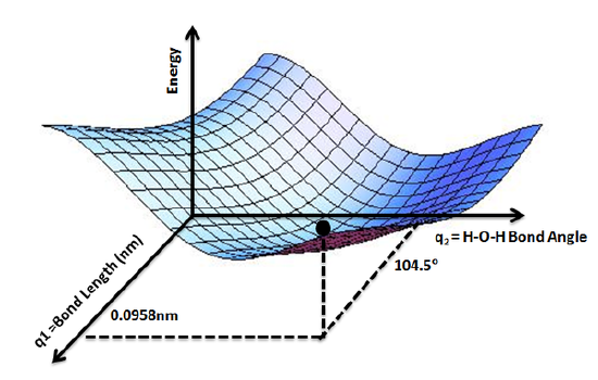
Figure \(\PageIndex{1}\): PES for water molecule showing the energy minimum corresponding to optimized molecular structure for water- O-H bond lengths of 0.0958nm and H-O-H bond angle of 104.5°. of Wikipedia (CC-BY-SA, Aimnature, Wikipedia).
PES depends on Born-Oppenheimer approximation, which states that the nuclei in a molecule are essentially stationary compared to the electrons. This approximation is significant in computational chemistry as it simplifies the application of Schrödinger equation to molecules by focusing on the electronic energy and adding in the nuclear repulsion energy. Inherently a classical construct with respect to the nuclei.
We always want to reach minimum on the PES - as molecules want to be at the lowest possible potential energy. A minimum on the PES is defined by curvatures that are all positives. A saddle point is characterized by a negative curvature in one direction and positive curvature in all other directions.
At the minima and saddle point, the slope of the function is set to zero, where
\[ (\frac{df}{dx})_y = 0 , (\frac{df}{dy})_x = 0 $$ .
At the minima, the second derivatives are positive, due to positive curvature, that is
\[ (\frac{d^2f}{dx^2})_y = > 0 $$ , $$ (\frac{d^2f}{dy^2})_x = > 0 $$ .
And at the saddle point, one of the second derivative is negative (negative curvature), and all other derivatives are positives, so that
\[ (\frac{d^2f}{dx^2})_y = < 0 \[ , $$ (\frac{d^2f}{dy^2})_x = > 0 \]
The model surface: \(H+ H_2\)
Three dimensional PES is used for triatomic systems by substituting the collision reaction of an atom with a diatomic molecule. The very first study done on this topic is \(H_3\) atom. The reaction is
\[ H + H_2 \rightarrow H_2 + H \]
In this case, the triatomic molecule is the H-H-H transition state. The potential energy surface at this point will have a barrier as it has a higher energy than the reactants or products. Quantum mechanical and quasiclassical trajectories calculations require the PES for the H3 system. The PES does not dependent on the masses of the atoms, thus, the H3 surface can be used for any isotopic variant of this reaction. As three nuclei (ABC) are involved, the PES depends on three coordinates. Therefore, one coordinate needs to be fixed in order to plot the PES as a function of the remaining two.
The potential energy surface of \(H + H_2\) can be seen in figure below


Figure \(\PageIndex{2}\): (left) The potential energy contour map for the exchange reaction \(H_A + H_BH_C → H_AH_B + H_C\). The x-axis is \(R_{AB}\), the interatomic distance between \(H_A \, \ce{and} \, H_B\). These two atoms begin very far apart, but end up being bonded together. The y-axis is \(R_{BC}\), the interatomic distance between \(H_B \, \ce{and} \, H_C\). These two atoms start out bonded together but end up separated and far apart. The darker the color, the lower the potential energy. (right) The 3-D potential energy surface for the exchange reaction \(H_A + H_BH_C → H_AH_B + H_C\). The darker the color, the lower the potential energy. (CC BY-NC; Ümit Kaya via LibreTexts)
(Potential energy surface for the \(H_3 (H+H_2)\) system (Springer, 1998))
The three dimensional potential energy surfaces can be seen in this contour plot, where A-B-C transition state is marked by a red dot.

Figure \(\PageIndex{3}\): An energy contour map showing three possible reaction pathways for the reaction \[H_A + H_BH_C \rightarrow H_AH_B + H_C \nonumber \] (CC BY-NC; Ümit Kaya via LibreTexts)
The barrier at the transition state is called the saddle point, a minimum along the symmetric stretch coordinates, but a maximum along the asymmetric stretching coordinates.