Where is the electron in a hydrogen atom?
- Page ID
- 50010
\( \newcommand{\vecs}[1]{\overset { \scriptstyle \rightharpoonup} {\mathbf{#1}} } \)
\( \newcommand{\vecd}[1]{\overset{-\!-\!\rightharpoonup}{\vphantom{a}\smash {#1}}} \)
\( \newcommand{\dsum}{\displaystyle\sum\limits} \)
\( \newcommand{\dint}{\displaystyle\int\limits} \)
\( \newcommand{\dlim}{\displaystyle\lim\limits} \)
\( \newcommand{\id}{\mathrm{id}}\) \( \newcommand{\Span}{\mathrm{span}}\)
( \newcommand{\kernel}{\mathrm{null}\,}\) \( \newcommand{\range}{\mathrm{range}\,}\)
\( \newcommand{\RealPart}{\mathrm{Re}}\) \( \newcommand{\ImaginaryPart}{\mathrm{Im}}\)
\( \newcommand{\Argument}{\mathrm{Arg}}\) \( \newcommand{\norm}[1]{\| #1 \|}\)
\( \newcommand{\inner}[2]{\langle #1, #2 \rangle}\)
\( \newcommand{\Span}{\mathrm{span}}\)
\( \newcommand{\id}{\mathrm{id}}\)
\( \newcommand{\Span}{\mathrm{span}}\)
\( \newcommand{\kernel}{\mathrm{null}\,}\)
\( \newcommand{\range}{\mathrm{range}\,}\)
\( \newcommand{\RealPart}{\mathrm{Re}}\)
\( \newcommand{\ImaginaryPart}{\mathrm{Im}}\)
\( \newcommand{\Argument}{\mathrm{Arg}}\)
\( \newcommand{\norm}[1]{\| #1 \|}\)
\( \newcommand{\inner}[2]{\langle #1, #2 \rangle}\)
\( \newcommand{\Span}{\mathrm{span}}\) \( \newcommand{\AA}{\unicode[.8,0]{x212B}}\)
\( \newcommand{\vectorA}[1]{\vec{#1}} % arrow\)
\( \newcommand{\vectorAt}[1]{\vec{\text{#1}}} % arrow\)
\( \newcommand{\vectorB}[1]{\overset { \scriptstyle \rightharpoonup} {\mathbf{#1}} } \)
\( \newcommand{\vectorC}[1]{\textbf{#1}} \)
\( \newcommand{\vectorD}[1]{\overrightarrow{#1}} \)
\( \newcommand{\vectorDt}[1]{\overrightarrow{\text{#1}}} \)
\( \newcommand{\vectE}[1]{\overset{-\!-\!\rightharpoonup}{\vphantom{a}\smash{\mathbf {#1}}}} \)
\( \newcommand{\vecs}[1]{\overset { \scriptstyle \rightharpoonup} {\mathbf{#1}} } \)
\(\newcommand{\longvect}{\overrightarrow}\)
\( \newcommand{\vecd}[1]{\overset{-\!-\!\rightharpoonup}{\vphantom{a}\smash {#1}}} \)
\(\newcommand{\avec}{\mathbf a}\) \(\newcommand{\bvec}{\mathbf b}\) \(\newcommand{\cvec}{\mathbf c}\) \(\newcommand{\dvec}{\mathbf d}\) \(\newcommand{\dtil}{\widetilde{\mathbf d}}\) \(\newcommand{\evec}{\mathbf e}\) \(\newcommand{\fvec}{\mathbf f}\) \(\newcommand{\nvec}{\mathbf n}\) \(\newcommand{\pvec}{\mathbf p}\) \(\newcommand{\qvec}{\mathbf q}\) \(\newcommand{\svec}{\mathbf s}\) \(\newcommand{\tvec}{\mathbf t}\) \(\newcommand{\uvec}{\mathbf u}\) \(\newcommand{\vvec}{\mathbf v}\) \(\newcommand{\wvec}{\mathbf w}\) \(\newcommand{\xvec}{\mathbf x}\) \(\newcommand{\yvec}{\mathbf y}\) \(\newcommand{\zvec}{\mathbf z}\) \(\newcommand{\rvec}{\mathbf r}\) \(\newcommand{\mvec}{\mathbf m}\) \(\newcommand{\zerovec}{\mathbf 0}\) \(\newcommand{\onevec}{\mathbf 1}\) \(\newcommand{\real}{\mathbb R}\) \(\newcommand{\twovec}[2]{\left[\begin{array}{r}#1 \\ #2 \end{array}\right]}\) \(\newcommand{\ctwovec}[2]{\left[\begin{array}{c}#1 \\ #2 \end{array}\right]}\) \(\newcommand{\threevec}[3]{\left[\begin{array}{r}#1 \\ #2 \\ #3 \end{array}\right]}\) \(\newcommand{\cthreevec}[3]{\left[\begin{array}{c}#1 \\ #2 \\ #3 \end{array}\right]}\) \(\newcommand{\fourvec}[4]{\left[\begin{array}{r}#1 \\ #2 \\ #3 \\ #4 \end{array}\right]}\) \(\newcommand{\cfourvec}[4]{\left[\begin{array}{c}#1 \\ #2 \\ #3 \\ #4 \end{array}\right]}\) \(\newcommand{\fivevec}[5]{\left[\begin{array}{r}#1 \\ #2 \\ #3 \\ #4 \\ #5 \\ \end{array}\right]}\) \(\newcommand{\cfivevec}[5]{\left[\begin{array}{c}#1 \\ #2 \\ #3 \\ #4 \\ #5 \\ \end{array}\right]}\) \(\newcommand{\mattwo}[4]{\left[\begin{array}{rr}#1 \amp #2 \\ #3 \amp #4 \\ \end{array}\right]}\) \(\newcommand{\laspan}[1]{\text{Span}\{#1\}}\) \(\newcommand{\bcal}{\cal B}\) \(\newcommand{\ccal}{\cal C}\) \(\newcommand{\scal}{\cal S}\) \(\newcommand{\wcal}{\cal W}\) \(\newcommand{\ecal}{\cal E}\) \(\newcommand{\coords}[2]{\left\{#1\right\}_{#2}}\) \(\newcommand{\gray}[1]{\color{gray}{#1}}\) \(\newcommand{\lgray}[1]{\color{lightgray}{#1}}\) \(\newcommand{\rank}{\operatorname{rank}}\) \(\newcommand{\row}{\text{Row}}\) \(\newcommand{\col}{\text{Col}}\) \(\renewcommand{\row}{\text{Row}}\) \(\newcommand{\nul}{\text{Nul}}\) \(\newcommand{\var}{\text{Var}}\) \(\newcommand{\corr}{\text{corr}}\) \(\newcommand{\len}[1]{\left|#1\right|}\) \(\newcommand{\bbar}{\overline{\bvec}}\) \(\newcommand{\bhat}{\widehat{\bvec}}\) \(\newcommand{\bperp}{\bvec^\perp}\) \(\newcommand{\xhat}{\widehat{\xvec}}\) \(\newcommand{\vhat}{\widehat{\vvec}}\) \(\newcommand{\uhat}{\widehat{\uvec}}\) \(\newcommand{\what}{\widehat{\wvec}}\) \(\newcommand{\Sighat}{\widehat{\Sigma}}\) \(\newcommand{\lt}{<}\) \(\newcommand{\gt}{>}\) \(\newcommand{\amp}{&}\) \(\definecolor{fillinmathshade}{gray}{0.9}\)When the wavefunctions that solve Schrödinger's equation \(\psi(x,y,z)\) are expressed in spherical coordinates, then the wavefunctions can be separated into a radial and angular components
\[ \psi(r,\theta,\phi) =R(r) Y(\theta, \phi) \label{1.1}\]
The \(Y (\theta , \varphi )\) functions provide information about where the electron is around the proton and the radial function \(R(r)\) describes how far the electron is away from the proton. Both \(R(r)\) and \(Y (\theta , \varphi )\) depend on all three quantum numbers \(n, l, m_l\), although energy of each wavefunction (\(E_n\)) depends on only \(n\).
In general, the radial wavefunction (\(R(r)\)) can be expressed as
\[ R(r) = Q(r) e^{-r/a} \label{1.2}\]
where \(Q(r)\) is a polynomial. \(R(r)\) is typically normalized so that it can used to calculate electron probability just like proper wavefunction (but only with respect to the radial, \(r\) dimension only). A more complete 3D description requires addressing the complete wavefunction in Equation \(\ref{1.1}\).
Since the square of a particle's wave function at some location yields the probability that the particle is at that location, one might think that we can determine the probability that the electron is within some range of radii by integrating; however this is incorrect.
\[ P ( r_1 < r < r_2) \neq \int_{r_1}^{r_2} R(r)^2 dr = \int_{r_1}^{r_2} Q(r)^2 e^{-2r/a} dr \label{1.3}\]
The trouble is that once we leave the familiar territory of Cartesian coordinates and venture into the Land of Spherical Coordinates, the volume element changes.
"Volumes" in One Dimension
In one dimension, things are dead simple: a single coordinate x describes everything. If we want to integrate, we must move a little extra distance in all dimensions ... which means a little extra distance dx. That's all there is.

The "differential volume element" is simply
\[ dV = dx\]
Actually this is the differential length element, but the connection to volume is better described below.
"Volumes" in Two Dimensions
In two dimensions, thing are more interesting because there are several ways to identify a location in space. The Cartesian system uses variables x and y.
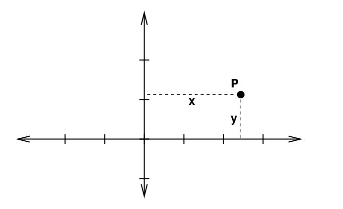
To integrate, we move a little extra distance in each dimension:

This sweeps out a little square box.
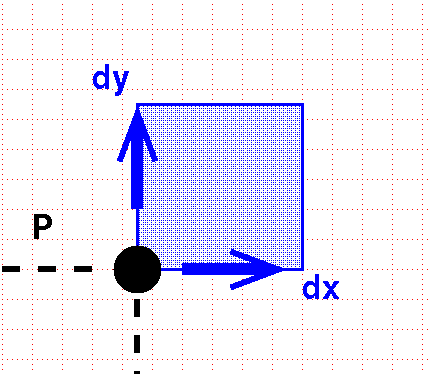
The differential volume element is the area of this box:
\[ dV = dx\, dy\]
Actually, this is the differential area element, but the connection to volume is described below.
Now, we can also use polar coordinates r and θ to describe the location of a point in a plane.

If we increase each of these variables by a teeny bit to integrate ...
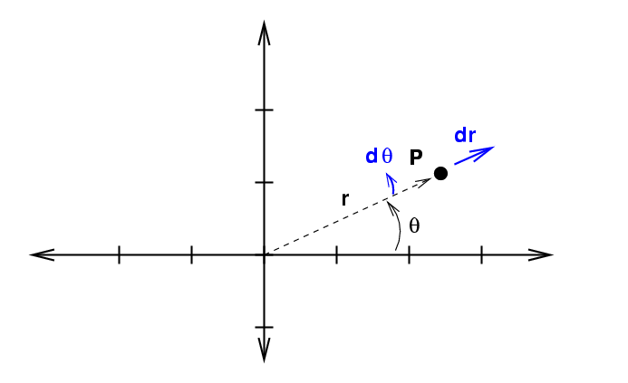
... we sweep out an area which is not square. Instead, it has a curve along the inside and outside edges.
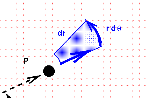
The area of this curvy box, and thus the differential volume element in polar coordinates on a plane, is
\[ dV = dr\, r d\theta\]
Actually, this is the differential area element.
Volumes in Three dimensions
I hope you'll believe me when I say that the differential volume element in three-dimensional Cartesian coordinates is
\[dV = dx\,dx\,dz\]
On the other hand, in three-dimensional spherical coordinates, we describe the position of an object with radius \(r\) and the angles \(θ\) and \(φ\).
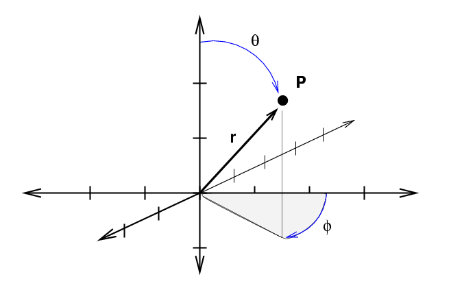
If we extend each of these three variables just a bit, we sweep out a funnel-shaped box.
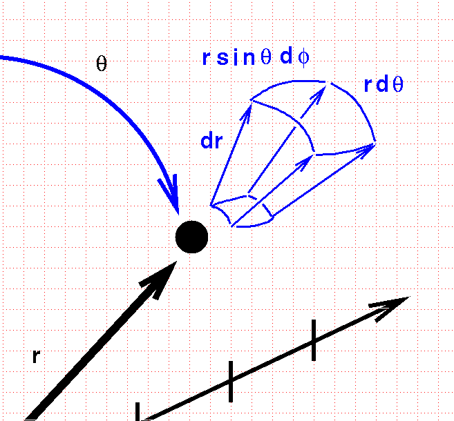
In one direction, the box has straight lines of length dr. In the other directions, the edges are curved. We can compute the length of these tiny arcs using the arclength formulae in spherical coordinates, and end up with a differential volume element
\[ dV = (dr) (rd\theta)(r \sin \theta \,d \phi)\]
\[ = r^2 \sin \theta \, dr\, d \theta \, d \phi\]
So, back to the electron within the hydrogen atom. The probability the electron is at location \((r, θ, φ)\) within a tolerance of \((dr, dθ, dφ)\) is
\[ P ( r; \theta; \phi) = \int (\psi( r; \theta; \phi))^2 dV\]
\[ P ( r; \theta; \phi) = \int (\psi( r; \theta; \phi))^2 r^2 \sin \theta \, dr\, d \theta \, d \phi \label{Int1}\]
If we can separate the wavefunction \(\ref{1.1}\) further into the product of three functions, each one dealing with only a single variable,
\[ \psi(r,\theta,\phi) =R(r) \Theta(\theta) \Phi(\phi) \]
then the integral in Equation \(\ref{Int1}\) becomes
\[ P ( r; \theta; \phi) = \int ( R(r) \Theta(\theta) \Phi(\phi) )^2 r^2 \sin \theta \, dr\, d \theta \, d \phi \label{Int2}\]
\[ = \int (R(r)^2 r^2 dr) (\Theta(\theta)^2 \sin \theta d \theta ) ( \Phi(\phi)^2 d \phi) \label{Int3}\]
\[ = \int R(r)^2 r^2 dr \int \Theta(\theta)^2 \sin \theta d \theta \int \Phi(\phi)^2 d \phi \label{Int4}\]
In the simplest case, corresponding to the ground state \(1s\), the wave function does not depend on either angle. That means the angular functions in Equation \(\ref{Int4}\) are simply equal to 1; and that makes doing those integrals trivial.
\[ \int 1 \sin \theta d\theta \label{Int5}\]
\[ \int 1 d\phi \label{Int6}\]
What are the limits and values of the integrals in Equations \(\ref{Int5}\) and \(\ref{Int6}\)?
So the probability of finding the electron within some range of radii (Equation \(\ref{1.3}\)) becomes
\[ P ( r_1 < r < r_2) = 4\pi \int_{r_1}^{r_2} R(r)^2 r^2 dr \label{Int7}\]
Recall that the radial function (Equation \(\ref{1.2}\)) can be separated into two compontents. For the electron in the 1s wavefunction, \(Q\) is a constant and then
\[ R(r) = Q e^{-r/a}\]
We can simplify this just a little bit by making a substitution: let
\[u = \dfrac{2r}{a}.\]
then
\[ du =\dfrac{2}{a} dr\]
and Equation \(\ref{Int7}\) can be rewritten as
\[ P ( r_1 < r < r_2) = 4\pi \left(Q^2 \dfrac{a^3}{8} \right) \int_{2r_1/a}^{2r_2/a} u^2 e ^{-u} du \label{Int8a}\]
You can look up that integral in a table; the result isn't too ugly.
\[ P ( r_1 < r < r_2) = 4\pi \left(Q^2 \dfrac{a^3}{8} \right) \left[ -e^{-u}(u^2 + 2u +2) \right]_{2r_1/a}^{2r_2/a} \label{Int9a}\]
- If we compute the probability that the radial position of the electron must be between zero and infinity, what must we get?
- Can you solve for the value of the coefficient \(Q\) in our radial wave function (for the 1s orbital)?
Visualizing Radial Probabilities
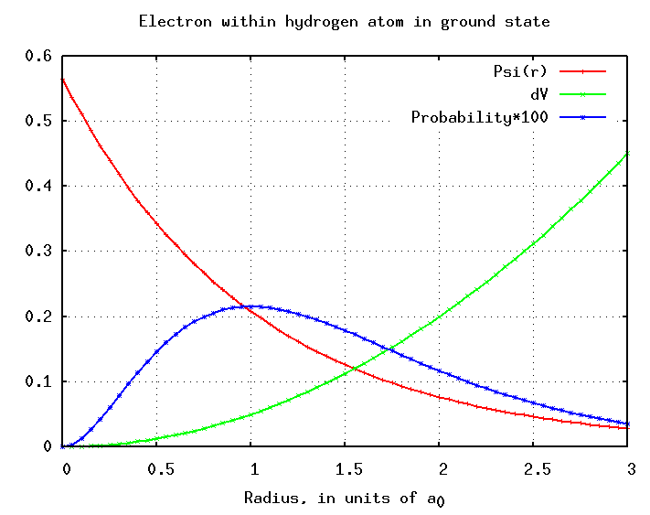
So, where is the electron most likely to be? While the \(R^2(r)\) plot (Figure 1; red curve) tracks the probability along a vector away from the nucleus, the \(r^2r^2(r)\) plot (blue curve) tracks the probability of a finding the electron at a radius \(r\). The peak of this curve is the MOST LIKELY radius for the electron.
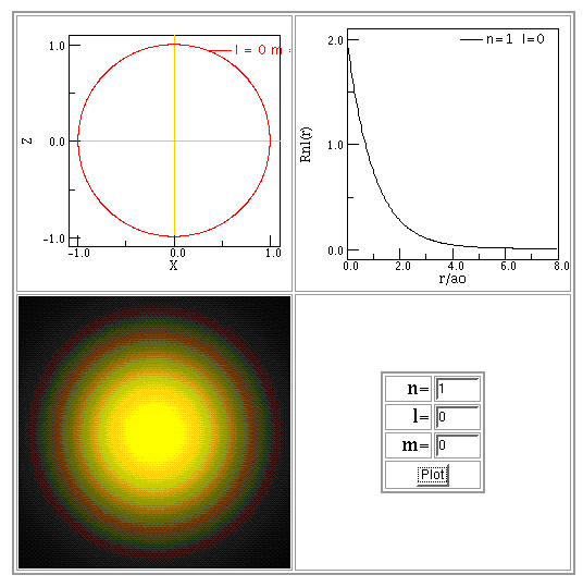
You can find more examples of wave functions and probability distributions in textbooks and on web sites. Below are some examples made using Paul Fastad's hydrogen atom applet. In each example, the radial function is shown in the top-right panel of the figure below, labelled "Rnl(r)". The bottom-left panel provides an illustration of this function, looking down at the atom from above.
