
Chapter 7. Hydrogen Atom
- Page ID
- 8856
\( \newcommand{\vecs}[1]{\overset { \scriptstyle \rightharpoonup} {\mathbf{#1}} } \)
\( \newcommand{\vecd}[1]{\overset{-\!-\!\rightharpoonup}{\vphantom{a}\smash {#1}}} \)
\( \newcommand{\id}{\mathrm{id}}\) \( \newcommand{\Span}{\mathrm{span}}\)
( \newcommand{\kernel}{\mathrm{null}\,}\) \( \newcommand{\range}{\mathrm{range}\,}\)
\( \newcommand{\RealPart}{\mathrm{Re}}\) \( \newcommand{\ImaginaryPart}{\mathrm{Im}}\)
\( \newcommand{\Argument}{\mathrm{Arg}}\) \( \newcommand{\norm}[1]{\| #1 \|}\)
\( \newcommand{\inner}[2]{\langle #1, #2 \rangle}\)
\( \newcommand{\Span}{\mathrm{span}}\)
\( \newcommand{\id}{\mathrm{id}}\)
\( \newcommand{\Span}{\mathrm{span}}\)
\( \newcommand{\kernel}{\mathrm{null}\,}\)
\( \newcommand{\range}{\mathrm{range}\,}\)
\( \newcommand{\RealPart}{\mathrm{Re}}\)
\( \newcommand{\ImaginaryPart}{\mathrm{Im}}\)
\( \newcommand{\Argument}{\mathrm{Arg}}\)
\( \newcommand{\norm}[1]{\| #1 \|}\)
\( \newcommand{\inner}[2]{\langle #1, #2 \rangle}\)
\( \newcommand{\Span}{\mathrm{span}}\) \( \newcommand{\AA}{\unicode[.8,0]{x212B}}\)
\( \newcommand{\vectorA}[1]{\vec{#1}} % arrow\)
\( \newcommand{\vectorAt}[1]{\vec{\text{#1}}} % arrow\)
\( \newcommand{\vectorB}[1]{\overset { \scriptstyle \rightharpoonup} {\mathbf{#1}} } \)
\( \newcommand{\vectorC}[1]{\textbf{#1}} \)
\( \newcommand{\vectorD}[1]{\overrightarrow{#1}} \)
\( \newcommand{\vectorDt}[1]{\overrightarrow{\text{#1}}} \)
\( \newcommand{\vectE}[1]{\overset{-\!-\!\rightharpoonup}{\vphantom{a}\smash{\mathbf {#1}}}} \)
\( \newcommand{\vecs}[1]{\overset { \scriptstyle \rightharpoonup} {\mathbf{#1}} } \)
\( \newcommand{\vecd}[1]{\overset{-\!-\!\rightharpoonup}{\vphantom{a}\smash {#1}}} \)
\(\newcommand{\avec}{\mathbf a}\) \(\newcommand{\bvec}{\mathbf b}\) \(\newcommand{\cvec}{\mathbf c}\) \(\newcommand{\dvec}{\mathbf d}\) \(\newcommand{\dtil}{\widetilde{\mathbf d}}\) \(\newcommand{\evec}{\mathbf e}\) \(\newcommand{\fvec}{\mathbf f}\) \(\newcommand{\nvec}{\mathbf n}\) \(\newcommand{\pvec}{\mathbf p}\) \(\newcommand{\qvec}{\mathbf q}\) \(\newcommand{\svec}{\mathbf s}\) \(\newcommand{\tvec}{\mathbf t}\) \(\newcommand{\uvec}{\mathbf u}\) \(\newcommand{\vvec}{\mathbf v}\) \(\newcommand{\wvec}{\mathbf w}\) \(\newcommand{\xvec}{\mathbf x}\) \(\newcommand{\yvec}{\mathbf y}\) \(\newcommand{\zvec}{\mathbf z}\) \(\newcommand{\rvec}{\mathbf r}\) \(\newcommand{\mvec}{\mathbf m}\) \(\newcommand{\zerovec}{\mathbf 0}\) \(\newcommand{\onevec}{\mathbf 1}\) \(\newcommand{\real}{\mathbb R}\) \(\newcommand{\twovec}[2]{\left[\begin{array}{r}#1 \\ #2 \end{array}\right]}\) \(\newcommand{\ctwovec}[2]{\left[\begin{array}{c}#1 \\ #2 \end{array}\right]}\) \(\newcommand{\threevec}[3]{\left[\begin{array}{r}#1 \\ #2 \\ #3 \end{array}\right]}\) \(\newcommand{\cthreevec}[3]{\left[\begin{array}{c}#1 \\ #2 \\ #3 \end{array}\right]}\) \(\newcommand{\fourvec}[4]{\left[\begin{array}{r}#1 \\ #2 \\ #3 \\ #4 \end{array}\right]}\) \(\newcommand{\cfourvec}[4]{\left[\begin{array}{c}#1 \\ #2 \\ #3 \\ #4 \end{array}\right]}\) \(\newcommand{\fivevec}[5]{\left[\begin{array}{r}#1 \\ #2 \\ #3 \\ #4 \\ #5 \\ \end{array}\right]}\) \(\newcommand{\cfivevec}[5]{\left[\begin{array}{c}#1 \\ #2 \\ #3 \\ #4 \\ #5 \\ \end{array}\right]}\) \(\newcommand{\mattwo}[4]{\left[\begin{array}{rr}#1 \amp #2 \\ #3 \amp #4 \\ \end{array}\right]}\) \(\newcommand{\laspan}[1]{\text{Span}\{#1\}}\) \(\newcommand{\bcal}{\cal B}\) \(\newcommand{\ccal}{\cal C}\) \(\newcommand{\scal}{\cal S}\) \(\newcommand{\wcal}{\cal W}\) \(\newcommand{\ecal}{\cal E}\) \(\newcommand{\coords}[2]{\left\{#1\right\}_{#2}}\) \(\newcommand{\gray}[1]{\color{gray}{#1}}\) \(\newcommand{\lgray}[1]{\color{lightgray}{#1}}\) \(\newcommand{\rank}{\operatorname{rank}}\) \(\newcommand{\row}{\text{Row}}\) \(\newcommand{\col}{\text{Col}}\) \(\renewcommand{\row}{\text{Row}}\) \(\newcommand{\nul}{\text{Nul}}\) \(\newcommand{\var}{\text{Var}}\) \(\newcommand{\corr}{\text{corr}}\) \(\newcommand{\len}[1]{\left|#1\right|}\) \(\newcommand{\bbar}{\overline{\bvec}}\) \(\newcommand{\bhat}{\widehat{\bvec}}\) \(\newcommand{\bperp}{\bvec^\perp}\) \(\newcommand{\xhat}{\widehat{\xvec}}\) \(\newcommand{\vhat}{\widehat{\vvec}}\) \(\newcommand{\uhat}{\widehat{\uvec}}\) \(\newcommand{\what}{\widehat{\wvec}}\) \(\newcommand{\Sighat}{\widehat{\Sigma}}\) \(\newcommand{\lt}{<}\) \(\newcommand{\gt}{>}\) \(\newcommand{\amp}{&}\) \(\definecolor{fillinmathshade}{gray}{0.9}\)Atomic Spectra
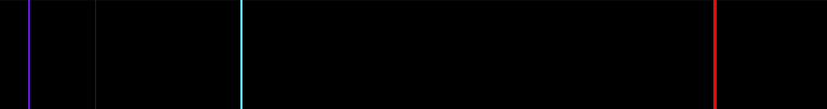
When gaseous hydrogen in a glass tube is excited by a \(5000\)-volt electrical discharge, four lines are observed in the visible part of the emission spectrum: red at \(656.3\) nm, blue-green at \(486.1\) nm, blue violet at \(434.1\) nm and violet at \(410.2\) nm:
Other series of lines have been observed in the ultraviolet and infrared regions. Rydberg (1890) found that all the lines of the atomic hydrogen spectrum could be fitted to a single formula
\[ \dfrac{1}{\lambda} = \mathcal{R} \left( \dfrac{1}{n_1^{2}} - \dfrac{1}{n_2^{2}} \right), \quad n_1 = 1, \: 2, \: 3..., \: n_2 > n_1 \label{1}\]
where \(\mathcal{R}\), known as the Rydberg constant, has the value \(109,677\) cm-1 for hydrogen. The reciprocal of wavelength, in units of cm-1, is in general use by spectroscopists. This unit is also designated wavenumbers, since it represents the number of wavelengths per cm. The Balmer series of spectral lines in the visible region, shown in Figure \(\PageIndex{1}\), correspond to the values \(n_1 = 2, \: n_2 = 3, \: 4, \: 5\) and \(6\). The lines with \(n_1 = 1\) in the ultraviolet make up the Lyman series. The line with \(n_2 = 2\), designated the Lyman alpha, has the longest wavelength (lowest wavenumber) in this series, with \(1/ \lambda = 82.258\) cm-1 or \(\lambda = 121.57\) nm.
Other atomic species have line spectra, which can be used as a "fingerprint" to identify the element. However, no atom other than hydrogen has a simple relation analogous to Equation \(\ref{1}\) for its spectral frequencies. Bohr in 1913 proposed that all atomic spectral lines arise from transitions between discrete energy levels, giving a photon such that
\[ \Delta E = h \nu = \dfrac{hc}{\lambda} \label{2}\]
This is called the Bohr frequency condition. We now understand that the atomic transition energy \(\Delta E\) is equal to the energy of a photon, as proposed earlier by Planck and Einstein.
The Bohr Atom
The nuclear model proposed by Rutherford in 1911 pictures the atom as a heavy, positively-charged nucleus, around which much lighter, negatively-charged electrons circulate, much like planets in the Solar system. This model is however completely untenable from the standpoint of classical electromagnetic theory, for an accelerating electron (circular motion represents an acceleration) should radiate away its energy. In fact, a hydrogen atom should exist for no longer than \(5 \times 10^{-11}\) sec, time enough for the electron's death spiral into the nucleus. This is one of the worst quantitative predictions in the history of physics. It has been called the Hindenberg disaster on an atomic level. (Recall that the Hindenberg, a hydrogen-filled dirigible, crashed and burned in a famous disaster in 1937.)
Bohr sought to avoid an atomic catastrophe by proposing that certain orbits of the electron around the nucleus could be exempted from classical electrodynamics and remain stable. The Bohr model was quantitatively successful for the hydrogen atom, as we shall now show.
We recall that the attraction between two opposite charges, such as the electron and proton, is given by Coulomb's law
\[F = \begin{cases} -\dfrac{e^{2}}{r^{2}} \quad \mathsf{(gaussian \: units)} \\ -\dfrac{e^{2}}{4 \pi \epsilon_0 r^{2}} \quad \mathsf{(SI \: units)} \end{cases} \label{3}\]
We prefer to use the Gaussian system in applications to atomic phenomena. Since the Coulomb attraction is a central force (dependent only on r), the potential energy is related by
\[F = -\dfrac{dV(r)}{dr} \label{4}\]
We find therefore, for the mutual potential energy of a proton and electron,
\[V(r) = -\dfrac{e^2}{r} \label{5}\]
Bohr considered an electron in a circular orbit of radius \(r\) around the proton. To remain in this orbit, the electron must be experiencing a centripetal acceleration
\[a = -\dfrac{v^{2}}{r} \label{6}\]
where \(v\) is the speed of the electron. Using Equations \(\ref{4}\) and \(\ref{6}\) in Newton's second law, we find
\[\dfrac{e^{2}}{r^{2}} = \dfrac{mv^{2}}{r} \label{7}\]
where \(m\) is the mass of the electron. For simplicity, we assume that the proton mass is infinite (actually \(m_p \approx 1836 m_e\)) so that the proton's position remains fixed. We will later correct for this approximation by introducing reduced mass. The energy of the hydrogen atom is the sum of the kinetic and potential energies:
\[E = T + V = \dfrac{1}{2} mv^{2} - \dfrac{e^{2}}{r} \label{8}\]
Using Equation \(\ref{7}\), we see that
\[T = -\dfrac{1}{2} V\ \qquad \mathsf{and} \qquad E = \dfrac{1}{2} V = -T \label{9}\]
This is the form of the virial theorem for a force law varying as \(r^{-2}\). Note that the energy of a bound atom is negative, since it is lower than the energy of the separated electron and proton, which is taken to be zero.
For further progress, we need some restriction on the possible values of \(r\) or \(v\). This is where we can introduce the quantization of angular momentum \(\mathbf{L} = \mathbf{r} \times \mathbf{p}\). Since \(\mathbf{p}\) is perpendicular to \(\mathbf{r}\), we can write simply
\[L = rp = mvr \label{10}\]
Using Equation \(\ref{9}\), we find also that
\[r = \dfrac{L^{2}}{me^{2}} \label{11}\]
We introduce angular momentum quantization, writing
\[L = n\hbar, \qquad n = 1, \: 2... \label{12}\]
excluding \(n = 0\), since the electron would then not be in a circular orbit. The allowed orbital radii are then given by
\[r_n = n^{2} a_0 \label{13}\]
where
\[a_0 \equiv \dfrac{\hbar^{2}}{me^{2}} = 5.29 \times 10^{-11} \: \mathsf{m} = 0.529Å \label{14}\]
which is known as the Bohr radius. The corresponding energy is
\[E_n = -\dfrac{e^{2}}{2a_0n^{2}} = -\dfrac{me^{4}}{2\hbar^{2}n^{2}}, \qquad n = 1, \: 2... \label{15}\]
Rydberg's formula (Equation \(\ref{1}\)) can now be deduced from the Bohr model. We have
\[ \dfrac{hc}{\lambda} = E_{n_2} - E_{n_1} = \dfrac{2\pi^{2}me^{4}}{h^{2}} \left( \dfrac{1}{n_1^{2}} - \dfrac{1}{n_2^{2}} \right) \label{16}\]
and the Rydbeg constant can be identified as
\[\mathcal{R} = \dfrac{2\pi^{2}me^{4}}{h^{3}c} \approx 109,737 \: \mathsf{cm}^{-1} \label{17}\]
The slight discrepency with the experimental value for hydrogen \( (109,677) \) is due to the finite proton mass. This will be corrected later.
The Bohr model can be readily extended to hydrogenlike ions, systems in which a single electron orbits a nucleus of arbitrary atomic number \(Z\). Thus \(Z = 1\) for hydrogen, \(Z = 2\) for \(\mathsf{He}^{+}\), \(Z = 3\) for \(\mathsf{Li}^{++}\), and so on. The Coulomb potential \(\ref{5}\) generalizes to
\[V(r) = -\dfrac{Ze^{2}}{r}, \label{18}\]
the radius of the orbit (Equation \(\ref{13}\)) becomes
\[r_n = \dfrac{n^{2}a_0}{Z} \label{19}\]
and the energy Equation \(\ref{15}\) becomes
\[E_n = -\dfrac{Z^{2}e^{2}}{2a_0n^{2}} \label{20}\]
De Broglie's proposal that electrons can have wavelike properties was actually inspired by the Bohr atomic model. Since
\[L = rp = n\hbar = \dfrac{nh}{2\pi} \label{21}\]
we find
\[2\pi r = \dfrac{nh}{p} = n\lambda \label{22}\]
Therefore, each allowed orbit traces out an integral number of de Broglie wavelengths.
Wilson (1915) and Sommerfeld (1916) generalized Bohr's formula for the allowed orbits to
\[\oint p \, dr = nh, \qquad n =1, \: 2... \label{23}\]
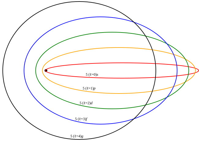
The Sommerfeld-Wilson quantum conditions Equation \(\ref{23}\) reduce to Bohr's results for circular orbits, but allow, in addition, elliptical orbits along which the momentum \(p\) is variable. According to Kepler's first law of planetary motion, the orbits of planets are ellipses with the Sun at one focus. Figure \(\PageIndex{2}\) shows the generalization of the Bohr theory for hydrogen, including the elliptical orbits. The lowest energy state \(n = 1\) is still a circular orbit. But \(n = 2\) allows an elliptical orbit in addition to the circular one; \(n = 3\) has three possible orbits, and so on. The energy still depends on \(n\) alone, so that the elliptical orbits represent degenerate states. Atomic spectroscopy shows in fact that energy levels with \(n > 1\) consist of multiple states, as implied by the splitting of atomic lines by an electric field (Stark effect) or a magnetic field (Zeeman effect). Some of these generalized orbits are drawn schematically in Figure \(\PageIndex{2}\).
The Bohr model was an important first step in the historical development of quantum mechanics. It introduced the quantization of atomic energy levels and gave quantitative agreement with the atomic hydrogen spectrum. With the Sommerfeld-Wilson generalization, it accounted as well for the degeneracy of hydrogen energy levels. Although the Bohr model was able to sidestep the atomic "Hindenberg disaster," it cannot avoid what we might call the "Heisenberg disaster." By this we mean that the assumption of well-defined electronic orbits around a nucleus is completely contrary to the basic premises of quantum mechanics. Another flaw in the Bohr picture is that the angular momenta are all too large by one unit, for example, the ground state actually has zero orbital angular momentum (rather than \(\hbar\)).
The assumption of well-defined electronic orbits around a nucleus in the Bohr atom is completely contrary to the basic premises of quantum mechanics.
Quantum Mechanics of Hydrogenlike Atoms
In contrast to the particle in a box and the harmonic oscillator, the hydrogen atom is a real physical system that can be treated exactly by quantum mechanics. In addition to their inherent significance, these solutions suggest prototypes for atomic orbitals used in approximate treatments of complex atoms and molecules.
For an electron in the field of a nucleus of charge \(+Ze\), the Schrӧdinger equation can be written
\[\left\{ -\dfrac{\hbar^{2}}{2m} \nabla^{2} - \dfrac{Ze^{2}}{r} \right\} \psi(r) = E\psi(r) \label{24}\]
It is convenient to introduce atomic units in which length is measured in bohrs:
\[a_0 = \dfrac{\hbar^{2}}{me^{2}} = 5.29 \times 10^{-11} \: \mathsf{m} \equiv 1 \: \mathsf{bohr} \]
and energy in hartrees:
\[\dfrac{e^2}{a_0} = 4.358 \times 10^{-18} \: \mathsf{J} = 27.211 \: \mathsf{eV} \equiv 1 \: \mathsf{hartree} \]
Electron volts \((\mathsf{eV})\) are a convenient unit for atomic energies. One \(\mathsf{eV}\) is defined as the energy an electron gains when accelerated across a potential difference of \(1 \: \mathsf{volt}\). The ground state of the hydrogen atom has an energy of \(-1/2 \: \mathsf{hartree}\) or \(-13.6 \: \mathsf{eV}\). Conversion to atomic units is equivalent to setting
\[\hbar = e = m = 1\]
in all formulas containing these constants. Rewriting the Schrӧdinger equation in atomic units, we have
\[\left\{ -\dfrac{1}{2} \nabla^{2} - \dfrac{Z}{r} \right\} \psi(r) = E\psi(r) \label{25}\]
Since the potential energy is spherically symmetrical (a function of \(r\) alone), it is obviously advantageous to treat this problem in spherical polar coordinates \(r, \: \theta, \: \phi\). Expressing the Laplacian operator in these coordinates [cf. Eq (6-20)],
\[ -\dfrac{1}{2} \left\{ \dfrac{1}{r^{2}} \dfrac{\partial}{\partial r} r^{2} \dfrac{\partial}{\partial r} + \dfrac{1}{r^{2}\sin\theta} \dfrac{\partial}{\partial \theta} \sin\theta \dfrac{\partial}{\partial \theta} + \dfrac{1}{r^{2}\sin^{2}\theta} \dfrac{\partial^{2}}{\partial\phi^{2}} \right\} \\ \times \psi(r, \: \theta, \: \phi) - \dfrac{Z}{r} \psi(r, \: \theta, \: \phi) = E\psi(r, \: \theta, \: \phi) \label{26}\]
Equation \(\ref{26}\) shows that the second and third terms in the Laplacian represent the angular momentum operator \(\hat{L}^{2}\). Clearly, Equation \(\ref{26}\) will have separable solutions of the form
\[\psi(r, \: \theta, \: \phi) = R(r)Y_{\ell m}(\theta, \: \phi) \label{27}\]
Substituting Equation \(\ref{27}\) into Equation \(\ref{26}\) and using the angular momentum eigenvalue Equation Equation \(\ref{6-34}\), we obtain an ordinary differential equation for the radial function \(R(r)\):
\[\left\{ -\dfrac{1}{2r^{2}} \dfrac{d}{dr} r^{2} \dfrac{d}{dr} + \dfrac{\ell(\ell + 1)}{2r^{2}} - \dfrac{Z}{r} \right\} R(r) = ER(r) \label{28}\]
Note that in the domain of the variable \(r\), the angular momentum contribution \(\ell (\ell + 1) / 2r^{2}\) acts as an effective addition to the potential energy. It can be identified with centrifugal force, which pulls the electron outward, in opposition to the Coulomb attraction. Carrying out the successive differentiations in Equation \(\ref{29}\) and simplifying, we obtain
\[\dfrac{1}{2}R''(r) + \dfrac{1}{r}R'(r) + \left[\dfrac{Z}{r} - \dfrac{\ell(\ell + 1)}{2r^{2}} + E\right]R(r) = 0 \label{29}\]
another second-order linear differential equation with non-constant coefficients. It is again useful to explore the asymptotic solutions to Equation \(\ref{29}\), as \(r \rightarrow \infty\). In the asymptotic approximation,
\[R''(r) - 2r\lvert E \rvert R(r) \approx 0 \label{30}\]
having noted that the energy \(E\) is negative for bound states. Solutions to Equation \(\ref{30}\) are
\[R(r) \approx \mathsf{const} \, e^{\pm\sqrt{2\lvert E \rvert}r} \label{31}\]
We reject the positive exponential on physical grounds, since \(R(r) \rightarrow \infty\) as \(r \rightarrow \infty\), in violation of the requirement that the wavefunction must be finite everywhere. Choosing the negative exponential and setting \(E = -Z^{2}/2\) the ground state energy in the Bohr theory (in atomic units), we obtain
\[R(r) \approx \mathsf{const} \, e^{-Zr} \label{32}\]
It turns out, very fortunately, that this asymptotic approximation is also an exact solution of the Schrӧdinger equation (Equation \(\ref{29}\)) with \(\ell = 0\), just what happened for the harmonic-oscillator problem in Chap. 5. The solutions to Equation \(\ref{29}\), designated \(R_{n\ell}(r)\), are labeled by \(n\), known as the principal quantum number, as well as by the angular momentum \(\ell\), which is a parameter in the radial equation. The solution in Equation \(\ref{32}\) corresponds to \(R_{10}(r)\). This should be normalized according to the condition
\[\int_{0}^{\infty} [R_{10}(r)]^{2} \, r^{2} \, dr = 1 \label{33}\]
A useful definite integral is
\[\int_{0}^{\infty} r^{n} \, e^{-\alpha r} \, dr = \dfrac{n!}{\alpha^{n + 1}} \label{34}\]
The normalized radial function is thereby given by
\[R_{10}(r) = 2Z^{3/2} e^{-Zr} \label{35}\]
Since this function is nodeless, we identify it with the ground state of the hydrogenlike atom. Multipyling Equation \(\ref{35}\) by the spherical harmonic \(Y_{00} = 1/ \sqrt{4\pi} \), we obtain the total wavefunction (Equation \(\ref{27}\))
\[\psi_{100}(r, \theta, \phi) = \left( \dfrac{Z^{3}}{\pi} \right)^{1/2} e^{-Zr} \label{36}\]
This is conventionally designated as the 1s function \(\psi_{1s}(r)\).
Integrals in spherical-polar coordinates over a spherically-symmetrical integrand (like the 1s orbital) can be significantly simplified. We can do the reduction
\[\int_{0}^{\infty} \int_{0}^{\pi} \int_{0}^{2\pi} f(r) \, r^{2} \, \sin\theta \, dr \, d\theta \, d\phi = \int_{0}^{\infty} f(r) \, 4\pi r^{2} \, dr \label{37}\]
since integration over \(\theta\) and \(\phi\) gives \(4\pi\), the total solid angle of a sphere. The normalization of the 1s wavefunction can thus be written as
\[\int_{0}^{\infty} [\psi_{1s}(r)]^{2} \, 4\pi r^{2} \, dr = 1 \label{38}\]
Hydrogen Atom Ground State
There are a number of different ways of representing hydrogen-atom wavefunctions graphically. We will illustrate some of these for the 1s ground state. In atomic units,
\[\psi_{1s}(r) = \dfrac{1}{\sqrt{\pi}}e^{-r} \label{39}\]
is a decreasing exponential function of a single variable \(r\), and is simply plotted in Figure 3.
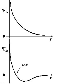
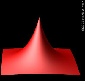
Figure \(\PageIndex{3}\) gives a somewhat more pictorial representation, a three-dimensional contour plot of \(\psi_{1s}(r)\) as a function of \(x\) and \(y\) in the \(x\), \(y\)-plane.
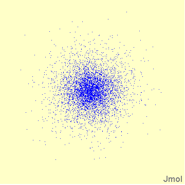
According to Born's interpretation of the wavefunction, the probability per unit volume of finding the electron at the point \((r, \: \theta, \: \phi) \) is equal to the square of the normalized wavefunction
\[\rho_{1s}(r) = [\psi_{1s}(r)]^{2} = \dfrac{1}{\pi}e^{-2r} \label{40}\]
This is represented in Figure 5 by a scatter plot describing a possible sequence of observations of the electron position. Although results of individual measurements are not predictable, a statistical pattern does emerge after a sufficiently large number of measurements.
The probability density is normalized such that
\[\int_{0}^{\infty} \rho_{1s}(r) \, 4\pi r^{2} \, dr = 1 \label{41}\]
In some ways \(\rho (r)\) does not provide the best description of the electron distribution, since the region around \(r = 0\), where the wavefunction has its largest values, is a relatively small fraction of the volume accessible to the electron. Larger radii \(r\) represent larger physical regions since, in spherical polar coordinates, a value of \(r\) is associated with a shell of volume \(4\pi r^{2} \, dr\). A more significant measure is therefore the radial distribution function
\[D_{1s}(r) = 4\pi r^{2} [\psi_{1s}(r)]^{2} \label{42}\]
which represents the probability density within the entire shell of radius \(r\), normalized such that
\[\int_{0}^{\infty} D_{1s}(r) \, dr = 1 \label{43}\]
The functions \(\rho_{1s}(r) \) and \(D_{1s}(r) \) are both shown in Figure \(\PageIndex{6}\). Remarkably, the 1s RDF has its maximum at \(r = a_0\), equal to the radius of the first Bohr orbit

Atomic Orbitals
The general solution for \(R_{n\ell}(r)\) has a rather complicated form which we give without proof:
\[R_{n\ell}(r) = N_{n\ell} \, \rho^{\ell} \, L_{n + \ell}^{2\ell + 1} \, (\rho) e^{-\rho /2} \qquad \rho \equiv \dfrac{2Zr}{n} \label{44}\]
Here \(L_{\beta}^{\alpha}\) is an associated Laguerre polynomial and \(N_{n\ell}\), a normalizing constant. The angular momentum quantum number \(\ell\) is by convention designated by a code: s for \(\ell\ = 0\), p for \(\ell\ = 1\), d for \(\ell\ = 2\), f for \(\ell\ = 3\), g for \(\ell\ = 4\), and so on. The first four letters come from an old classification scheme for atomic spectral lines: sharp, principal, diffuse and fundamental. Although these designations have long since outlived their original significance, they remain in general use. The solutions of the hydrogenic Schrӧdinger equation
in spherical polar coordinates can now be written in full
\[\psi_{n\ell m}(r, \: \theta, \: \phi) = R_{n\ell}(r)Y_{\ell m}(\theta, \: \phi) \\ n = 1, \: 2... \qquad \ell = 0, \: 1... \: n - 1 \qquad m = 0, \: \pm 1, \: \pm 2... \: \pm \ell \label{45}\]
where \(Y_{\ell m}\) are the spherical harmonics tabulated in Chap. 6. Table 1 below enumerates all the hydrogenic functions we will actually need. These are called hydrogenic atomic orbitals, in anticipation of their later applications to the structure of atoms and molecules.
| \[\psi_{1s} = \dfrac{1}{\sqrt{\pi}} e^{-r}\] |
| \[\psi_{2s} = \dfrac{1}{2\sqrt{2\pi}} \left( 1 - \dfrac{r}{2} \right) e^{-r/2}\] |
| \[\psi_{2p_z} = \dfrac{1}{4\sqrt{2\pi}} z \, e^{-r/2}\] |
| \[\psi_{2p_x}, \: \psi_{2p_y} \qquad \mathsf{analogous}\] |
| \[\psi_{3s} = \dfrac{1}{81\sqrt{3\pi}} (27 - 18r + 2r^{2}) e^{-r/3}\] |
| \[\psi_{3p_z} = \dfrac{\sqrt{2}}{81\sqrt{\pi}} (6 - r) z \, e^{-r/3}\] |
| \[\psi_{3p_x}, \: \psi_{3p_y} \qquad \mathsf{analogous}\] |
| \[\psi_{3d_{z^{2}}} = \dfrac{1}{81\sqrt{6\pi}}(3z^{2} - r^{2}) e^{-r/3}\] |
| \[\psi_{3d_{zx}} = \dfrac{\sqrt{2}}{81\sqrt{\pi}}zx \, e^{-r/3}\] |
| \[\psi_{3d_{yz}}, \: \psi_{3d_{xy}} \qquad \mathsf{analogous}\] |
| \[\psi_{3d_{x^{2} - y^{2}}} = \dfrac{1}{81\sqrt{\pi}}(x^{2} - y^{2}) e^{-r/3}\] |
The energy levels for a hydrogenic system are given by
\[E_n = -\dfrac{Z^{2}}{2n^{2}} \: \mathsf{hartrees} \label{46}\]
and depends on the principal quantum number alone. Considering all the allowed values of \(\ell\) and \(m\), the level \(E_n\) has a degeneracy of \(n^{2}\). Figure 7 shows an energy level diagram for hydrogen \((Z = 1) \). For \(E \geq 0\), the energy is a continuum, since the electron is in fact a free particle. The continuum represents states of an electron and proton in interaction, but not bound into a stable atom. Figure \(\PageIndex{7}\) also shows some of the transitions which make up the Lyman series in the ultraviolet and the Balmer series in the visible region.

The \(ns\) orbitals are all spherically symmetrical, being associated with a constant angular factor, the spherical harmonic \(Y_{00} = 1/ \sqrt{4\pi} \). They have \(n - 1\) radial nodes—spherical shells on which the wavefunction equals zero. The 1s ground state is nodeless and the number of nodes increases with energy, in a pattern now familiar from our study of the particle-in-a-box and harmonic oscillator. The 2s orbital, with its radial node at \(r = 2\) bohr, is also shown in Figure \(\PageIndex{3}\).
p- and d-Orbitals
The lowest-energy solutions deviating from spherical symmetry are the 2p-orbitals. Using Equations \(\ref{44}\), \(\ref{45}\) and the \(\ell = 1\) spherical harmonics, we find three degenerate eigenfunctions:
\[\psi_{210}(r, \: \theta, \: \phi) = \dfrac{1}{4\sqrt{2\pi}}re^{-r/2} \cos\theta \label{47}\]
and
\[\psi_{21 \pm 1}(r, \: \theta, \: \phi) = \mp \dfrac{1}{4\sqrt{2\pi}}re^{-r/2} \sin\theta e^{\pm i \phi} \label{48}\]
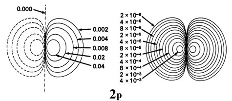
The function \(\psi_{210}\) is real and contains the factor \(r \cos\theta \), which is equal to the cartesian variable \(z\). In chemical applications, this is designated as a 2pz orbital:
\[\psi_{2p_z} = \dfrac{1}{4\sqrt{2\pi}}ze^{-r/2} \label{49}\]
A contour plot is shown in Figure \(\PageIndex{8}\). Note that this function is cylindrically-symmetrical about the \(z\)-axis with a node in the \(x\), \(y\)-plane. The \(\psi_{21 \pm 1}\) are complex functions and not as easy to represent graphically. Their angular dependence is that of the spherical harmonics \(Y_{1 \pm 1}\), shown in Figure 6-4. As noted in Chap. 4, any linear combination of degenerate eigenfunctions is an equally-valid alternative eigenfunction. Making use of the Euler formulas for sine and cosine
\[\cos\phi = \dfrac{e^{i\phi} + e^{-i\phi}}{2} \qquad \mathsf{and} \qquad \sin\phi = \dfrac{e^{i\phi} - e^{-i\phi}}{2} \label{50}\]
and noting that the combinations \(\sin\theta\cos\phi\) and \(\sin\theta\sin\phi\) correspond to the cartesian variables \(x\) and \(y\), respectively, we can define the alternative 2p orbitals
\[\psi_{2p_x} = \dfrac{1}{\sqrt{2}}(\psi_{21-1} - \psi_{211}) = \dfrac{1}{4\sqrt{2\pi}} xe^{-r/2} \label{51}\]
and
\[\psi_{2p_y} = -\dfrac{i}{\sqrt{2}}(\psi_{21-1} + \psi_{211}) = \dfrac{1}{4\sqrt{2\pi}} ye^{-r/2} \label{52}\]
Clearly, these have the same shape as the 2pz-orbital, but are oriented along the \(x\)- and \(y\)-axes, respectively. The threefold degeneracy of the p-orbitals is very clearly shown by the geometric equivalence the functions 2px, 2py and 2pz, which is not obvious for the spherical harmonics. The functions listed in Table 1 are, in fact, the real forms for all atomic orbitals, which are more useful in chemical applications. All higher p-orbitals have analogous functional forms \(x \, f(r)\), \(y \, f(r)\) and \(z \, f(r)\) and are likewise 3-fold degenerate.
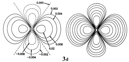
The orbital \(\psi_{320}\) is, like \(\psi_{210}\), a real function. It is known in chemistry as the \(d_{z^{2}}\)-orbital and can be expressed as a cartesian factor times a function of \(r\):
\[\psi_{3d_{z^{2}}} = \psi_{320} = (3z^{2} - r^{2}) f(r) \label{53}\]
A contour plot is shown in Figure \(\PageIndex{9}\). This function is also cylindrically symmetric about the \(z\)-axis with two angular nodes—the conical surfaces with \(3z^{2} - r^{2} = 0\). The remaining four 3d orbitals are complex functions containing the spherical harmonics \(Y_{2 \pm 1} \) and \(Y_{2 \pm 2}\) pictured in Figure 6-4. We can again construct real functions from linear combinations, the result being four geometrically equivalent "four-leaf clover" functions with two perpendicular planar nodes. These orbitals are designated \(d_{x^{2} - y^{2}}, \: d_{xy}, \: d_{zx}\) and \(d_{yz}\). Two of them are shown in Figure 9. The \(d_{z^{2}}\) orbital has a different shape. However, it can be expressed in terms of two non-standard d-orbitals, \(d_{z^{2} - x^{2}}\) and \(d_{y^{2} - z^{2}}\). The latter functions, along with \(d_{x^{2} - y^{2}}\) add to zero and thus constitute a linearly dependent set. Two combinations of these three functions can be chosen as independent eigenfunctions.
Summary
The atomic orbitals listed in Table 1 are illustrated in Figure \(\PageIndex{20}\). Blue and red indicate, respectively, positive and negative regions of the wavefunctions (the radial nodes of the 2s and 3s orbitals are obscured). These pictures are intended as stylized representations of atomic orbitals and should not be interpreted as quantitatively accurate.

The electron charge distribution in an orbital \(\psi_{n\ell m}(\mathbf{r})\) is given by
\[\rho(\mathbf{r}) = \lvert \psi_{n\ell m}(\mathbf{r}) \rvert ^{2} \label{54} \]
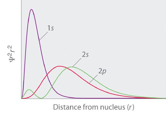
which for the s-orbitals is a function of \(r\) alone. The radial distribution function can be defined, even for orbitals containing angular dependence, by
\[D_{n\ell}(r) = r^{2} [R_{n\ell}(r)]^{2} \label{55}\]
This represents the electron density in a shell of radius \(r\), including all values of the angular variables \(\theta\), \(\phi\). Figure \(\PageIndex{11}\) shows plots of the RDF for the first few hydrogen orbitals.
Contributors and Attributions
Seymour Blinder (Professor Emeritus of Chemistry and Physics at the University of Michigan, Ann Arbor)
- Integrated by Daniel SantaLucia (Chemistry student at Hope College, Holland MI)