11.12: Thermodynamics and Kinetics

Most thermodynamics expression in textbooks are "intramural" relations. They tell us how to determine numerical values for unfamiliar quantities, such as \(ΔS\) and \(ΔG\) (Equation \ref{1a}-\ref{1d}) for example), or how one such quantity depends on another such quantity (Equation \ref{1c}-\ref{1d}).

\[ \Delta S = \frac{Q_{rev}}{T} \label{1a} \]

\[\Delta G^{ \circ} = -RT \ln K_{eq} \label{1b} \]

\[\Delta G = \Delta H - T \Delta S \label{1c} \]

\[\begin{bmatrix} \frac{\delta(\Delta G)}{\delta T} \end{bmatrix}_{P} = - \Delta S \label{1d} \]

Only a few thermodynamic expressions are "extramural" relations--ones that tell us immediately something about "directly measurable" or familiar quantities: how, for example, an equilibrium pressure P, or concentration N₂, or quotient of concentrations K or cell voltage ξ varies with temperature (Equations \ref{1a}-\ref{1d}).

\[\frac{dP}{dT}= \frac{Q}{T \Delta V} \label{2a} \]

\[\frac{dN_{2}}{dT_{fp}} = \frac{-Q}{RT^{2}_{nfp}} \label{2b} \]

\[\ln \frac{K_{2}}{K_{1}} = \frac{Q_{irrev}}{R} \left( \frac{1}{T_{1}} - \frac{1}{T_{2}} \right) \label{2c} \]

\[nF \frac{d \xi}{dT} = \frac{Q_{rev}}{T} \label{2d} \]

These extramural relations (Equation \ref{2a}-\ref{2d}) show how equilibrium parameters (P, N₂, K, ξ) must change with temperature if perpetual motion of the second kind is impossible. Perpetual motion of the second kind is production of work (an increase in energy of a mechanical system) solely at the expense of the energy of a thermal reservoir. In its net effect upon the environment, it is, with respect to energy transformations, precisely the opposite of friction.

The most general statement of the Second-Law like behavior of Nature states that any process whose net effect is precisely the opposite of friction -- or heat flow, or any natural event -- is impossible. From that statement can be developed by relatively long and mathematically demanding arguments, as shown in many physical chemistry texts, the extramural relations (Equation \ref{2a}-\ref{2d}).

It is the chief purpose of this paper to show that the Clapeyron equation (\ref{2a}), the colligative property relations (such as Equation \ref{2b}), van 't Hoff's relation (Equation \ref{2c}), Gibbs-Helmholtz-type equations (such as Equation \ref{2d}) and, also (discussed later), the osmotic pressure law (Equation 19), Boltzmann's factor (equation 25), and Carnot's theorem (equation 35) can be obtained directly from the laws of chemical kinetics, without the use of calculus.

Our kinetic derivations of the extramural relations of the thermodynamics are based on Arrhenius's rate-constant expression

\[k = A^{-ΔH^*/RT}. \nonumber \]

It will be shown that the derivations depend ultimately, therefore, on van 't Hoff's thermodynamic equilibrium-constant expression

\[K = C^{-ΔH/RT}. \label{therm} \]

Thus, the kinetic derivations are not, in a logical sense, a substitute for the usual thermodynamics arguments. It is often illuminating, however, to see abstract expressions (such as those of thermodynamics) emerge seemingly unexpectedly from more concrete equations (those of chemical kinetics).

The mathematical procedures in this paper can be used, also, in purely thermodynamic arguments. With no change in the algebraic steps given below, one can derive the extramural relations of thermodynamics directly from the thermodynamic expression in Equation \ref{therm}. Thus one can move rigorously and easily from one extramural relation to another without employing calculus and the entropy function (or the chemical potential), or Carnot cycles. This simplification of the syntax of thermodynamics serves to emphasize an essential point: there is essentially only one physically independent extramural thermodynamic relation. There is only one Second Law. Expressions (Equations \ref{2a}-\ref{2d}), the osmotic pressure rule (19), and Boltzmann's factor (25) are all special instances of Carnot's theorem (35).

In summary the present discussion is, simultaneously: a set of novel applications to thermodynamics of Arrhenius's rate-constant expression; a non-calculus review from several new points of view of the central expressions of classical (and, briefly, statistical) thermodynamics; and, in close, a brief account of the origins in kinetics and thermodynamics of activated complex theory.

Henry's Law and Raoult's Law

Many texts give this kinetic interpretation of Henry and Raoult laws. Consider the change

\[ x~(solution) \underset{k_b}{\stackrel{k_f}{\rightleftharpoons}} x~(gas) \nonumber \]

Let \(R_{f(b)}\) represent the rate of the forward (backward) reaction, specific rate constant k_f(b). Let \(C_x\) be the concentration (in any units) of \(X\) in the condensed phase, \(N_x\) its mole fraction therein, \(P_x\) its partial pressure in the gas phase, \(P^o_x\) the vapor pressure of pure \(X\). On the assumption that one has

\[R_{f} = k_{f}C_{x} \label{3a} \]

\[R_{c} = k_{b}P_{x^{'}} \label{3b} \]

that at equilibrium (R_f = R_b)

\[ P_{x} = \frac{k_{f}}{k_{b}} c_{x} = K_{eq} C_{x} \nonumber \]

\[ \underbrace{ K_{eq} = \frac{P_{x}}{C_{x}} = 1}_{\text{Henry's Law}} \label{4a} \]

\[= \underbrace{ \dfrac{P_{x}}{C_{x}} = N_{x} = 1}_{\text{Raoult's Law}} \label{4b} \]

\( \equiv P^{ \circ}_{X^{'}}\)

Similar derivations of mathematical expressions for other colligative properties can be achieved by introducing Arrhenius's expression for the dependence upon temperature (and pressure) of the specific rate constants \(k_f\) and \(k_b\).

Arrhenius's Rate-Constant Law

According to Arrhenius (in modern notation), for forward and backward reactions

\[ k=Ae^{- \Delta H^{*}/RT} \label{6} \]

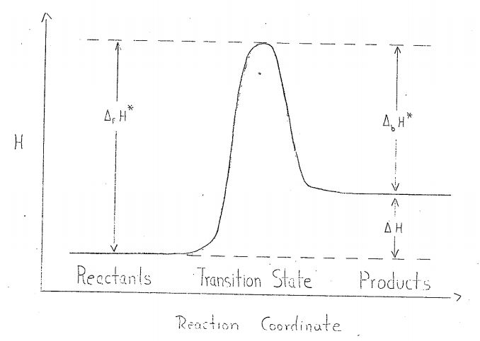
where, over small temperature intervals, \(A\) and \(ΔH^*\) may be treated as constants, and where, Fig. 1,

\[ \begin{align} \Delta_{f}H^{*} - \Delta_{b}H^{*} &= \Delta H \label{7a} \\ &= H_{products} - H_{reactions} \\[4pt] &= \Delta E + \Delta (PV). \label{7b} \end{align} \]

The Ideal Solubility Equation and Freezing Point Depression

To illustrate the use of the Arrhenius Rate-Constant Law to obtain by a kinetic analysis expressions normally obtained through reasoning based on thermodynamic principles, consider the solution, or melting, of a pure solid.

\[ x~(pure~solid) \underset{k_b}{\stackrel{k_f}{\rightleftharpoons}} x~(solution) \nonumber \]

On the assumption that R_f = k_f and R_b = k_bN_X, one has that, at equilibrium, k_f = k_bN_X or, on using the Arrhenius expression, (Equation \ref{6}), that

A_f^(-Δ_fH*/RT) = N_XA_b^(-Δ_bH*/RT).

Rearrangement and use of Equation \ref{7a} yields

\[ \frac{A_{f}}{A_{b}} = N_{x}e^{ \frac{ \Delta H}{RT}} \nonumber \]

ΔH is the enthalpy of solution, or melting, of X. Taking the natural logarithm of both sides of Equation \ref{8}, one obtains

\[ (a) \frac{ \Delta H}{RT} + \ln(N_{x}) = \ln( \frac{A_{f}}{A_{b}}) \nonumber \]

\( \ln( \frac{A_{f}}{A_{b}})\) is a constant

(b) \( \frac{ \Delta H}{RT} |_{N_{x} = 1}\)

(c) \( \frac{ \Delta H}{RT_{nfp}}\)

From (9c),

\[ \ln ( \frac{N_{x}}{1}) = \frac{ \Delta H}{R} \begin{pmatrix}
\frac{1}{T_{nfp}} & - & \frac{1}{T}
\end{pmatrix} \nonumber \]

For N_X ≈ 1, ln N_X ≈ -(1-N_X) ≡ -N₂, T ≈ T_nfp, and equation 10 reduces to

\[ N_{2} = \frac{- \Delta H}{RT^{2}nfp} (T-T_{nfp}) \nonumber \]

Equation 10, the ideal solubility equation, is a special case of equation 2c. Equation 11, the thermodynamic expression for freezing point depressions, is an integrated form of equation 2b.

Clapeyron's Equation

If a pure solid dissolves (melts) in its pure liquid,

\[ x~(pure~solid) \underset{k_b}{\stackrel{k_f}{\rightleftharpoons}} x~(pure~liquid) \nonumber \]

\(N_X = 1\) and, in place of Equation 9, one that has, at equilibrium, \( \frac{A_{f}}{A_{b}} = 1 \cdot ^{ \frac{ \Delta H}{RT}}\). Taking the natural logarithm of both sides, one obtains in place of Equation 9a

\[ \begin{align} \dfrac{ \Delta H}{RT} &= \ln \frac{A_{f}}{A_{b}}, \tag{a constant} \\[4pt] &= \dfrac{ \Delta E + P \Delta V}{RT} \label{13} \end{align} \]

Equation \ref{13} is obtained through equation 7b.

If the pressure and temperature change from values \(P\) and \(T\) that satisfy equation to new values \(P + dP\) and \(T + dT\), for equilibrium to be maintained, \(dP\) and \(dT\) must be such that

\[ \dfrac{ \Delta E + (P + dP) \Delta V}{R(T+dT)} = \frac{ \Delta E + P \Delta V}{RT} \label{14} \]

In writing Equation \ref{14}, it has been assumed that, like \( \frac{A_{f}}{A_{b}}\), \(ΔE\) and \(ΔV\) are temperature- and pressure-independent. Simplification of Equation \ref{14} yields, on solving for the ration of \(dP\) to \(dT\) in Equation \ref{2a} with

\[Q = ΔE + PΔV = ΔH. \nonumber \]

A kinetic analysis of the similar but slightly more complicated case of the vaporization of a liquid (or solid) is given in Appendix 1, together with a kinetic analysis of the effect on a vapor pressure of squeezing a liquid (the Gibbs-Poynting effect), with an application to osmosis.

Osmotic Equilibrium

Consider, next, diffusion of a pure solvent at pressure P through a rigid, semi-permeable membrane into a solution at pressure P + π,

\[ x~(pure~solvent) \underset{k_b}{\stackrel{k_f}{\rightleftharpoons}} x~(solution) \nonumber \]

	Pure Solvent	Solution
Pressure	P	P + π
Mole Fraction	NX = 1	NX < 1

The kinetic analysis R_f = k_f = R_b = k_bN_X yields with Arrhenius's relation, (6), expressions identical to (9) and (9a). In this instance, at least approximately, ΔE = ΔV = 0. Thus for (15)

\[ \Delta H = \Delta (PV) \ (P + \pi) \bar{V}_{x} - P \bar{V}_{x} = \pi \bar{V}_{x} \nonumber \]

Substitution from (16) into (9a) yields

\[ \frac{ \pi \bar{V}_{x}}{RT} + \ln(N_{x}) = \ln \frac{A_{f}}{A_{b}} \nonumber \]

where \( \ln (\frac{A_{f}}{A_{b}})\) is a constant.

For N_X = 1, π = 0 (at equilibrium). In this instance, therefore,

\[ \ln ( \frac{A_{f}}{A_{b}}) = 0 \nonumber \]

Substitution from (18) into (17) yields for dilute solutions (lnN_X ≈ -N₂) the usual thermodynamic expression for a solution's osmotic pressure π:

\[ \pi \approx \frac{RTN_{2}}{ bar{V}_{x}} \approx RTC_{2} \nonumber \]

in moles/liter.

Chemical Equilibrium

By the Principle of Microscopic Reversibility, one has that for chemical change

\[ aA + bB \underset{k_b}{\stackrel{k_f}{\rightleftharpoons}} dD + eE \nonumber \]

the rate at which A and B disappear by the (perhaps unlikely) mechanism aA + bB, rate law R_f = k_fc_A^ac_B^b, is at equilibrium equal to the rate at which A and B appear by the mechanism dD + eE, rate law R_b = k_bc_D^dc_E^e.¹ Thus, from R_b = R_f one obtains the familiar Law of Mass Action, equation 21 below, which with equations 6 and 7 yields equation 22, from which can be obtained directly equation 2c (Q_irrev = ΔH).

\[ \frac{C_{D}^{d}C_{E}^{e}}{C_{A}^{a}C_{B}^{b}} |_{equil.} = \frac{k_{f}}{k_{b}} = K_{eq} \nonumber \]

\[ = \frac{A_{f}}{A_{b}} e^{ \frac{- \Delta H}{RT}} \nonumber \]

For later reference, we note that, from equations 21 and 22,

\[ K_{eq} = \frac{A_{f}}{A_{b}} e^{ \frac{- \Delta H}{RT}} \nonumber \]

(b) \( e^{ \frac{ -[ \Delta H - RT \ln \frac{A_{f}}{A_{b}}]}{RT}}\)

¹For a further discussion of this point see: Frost, A. A., and Pearson, R. G., "Kinetics and Mechanism," John Wiley and Sons, Inc., 1953, Ch. 8; or Frost, A. A., J. Chem. Educ., 18, 272 (1941).

Boltzmann's Factor

A particularly simple "chemical" change is the transition of a molecule X in a quantum energy state i, energy ε_i, to a quantum energy state j, energy ε_j.

\[ x~(state~i) \underset{k_b}{\stackrel{k_f}{\rightleftharpoons}} x~(state~j) \nonumber \]

By arguments identical to those given in the preceding section, one obtains expressions of the form of equations 21 and 22. In this simple instance \( K_{eq} = \frac{C_{j}}{C_{i}}\) [C_j(i) = concentrations of molecules in state j (i)], ΔH = N_o (ε_j - ε_i) [Δ(PV) = 0\, and A_f = A_b. Thus, for a system that is at equilibrium with respect to the change indicated in equation 24,

\[ \frac{C_{j}}{C_{i}} = e^{ \frac{ -( \varepsilon_{j} - \varepsilon_{i} )}{kT}} \nonumber \]

where \(k \equiv \frac{R}{N_{o}}\)

From the Boltzmann factor expression, equation 25 can be obtained directly by summation partition functions and thence, by differentiation and the taking of logarithms, the other standard expressions of statistical thermodynamics.

Electrochemical Equilibrium

For the flow of electrons from a potential V₁ to a potential V₂,

\[ e~(potential~V_{1}) \underset{k_b}{\stackrel{k_f}{\rightleftharpoons}} e~(potential~V_{2}) \nonumber \]

in an electrochemical circuit, cell voltage ξ = V₂ - V₁, one has that at equilibrium (a "balanced circuit"), R_f = k_f = R_b = k_b. Thus, by the Arrhenius relation, equation 6, at equilibrium

\[ \frac{A_{f}}{A_{b}}=e^{ \frac{\Delta_{f} H^{*} - \Delta_{b} H^{*}}{RT}} \nonumber \]

The activation enthalpies of ΔH^{*} contain, in this instance, two contributions: one from the enthalpy of activation of the chemical change to which the electron flow is coupled in an electrochemical cell; the other from the enthalpy of activation for the physical transfer of electrons across a potential difference ξ. Thus, in this instance,

\[ (a) \frac{\Delta_{f} H^{*} - \Delta_{b} H^{*}}{RT} = \frac{ \Delta_{rx}H + nF \xi}{RT} \nonumber \]

\( = \ln \frac{A_{f}}{A_{b}}\), a constant (b)

At equilibrium the right-hand-side of (28) is equal to \( \ln \frac{A_{f}}{A_{b}}\), a constant, equation 28b. If the temperature and voltage change from values T and ξ that satisfy equations 28 to new values T + dT and ξ + dξ, for equilibrium to be maintained, dT and dξ must be such that

\[ \frac{ \Delta_{rx} H + nF ( \xi + d \xi)}{R(T + dT)} = \frac{ \Delta_{rx} H + nF \xi}{RT} \nonumber \]

In writing equation 29 it has been assumed (again) that, like \( \frac{A_{f}}{A_{b}}\), Δ_rxH is temperature independent: simplification of equation 29 yields on solving for the ratio of dξ to dT

\[ nf \frac{d \xi}{dT} = \frac{ \Delta_{rx} H + nF \xi}{T} \nonumber \]

Equation 30 is, in disguise, equation 2d. For consider this universe (or isolated system): a chemical system σ, an atmosphere atm, mechanical surroundings wt, and thermal surroundings θ [for example, as here, a chemical cell σ at constant temperature (owing to thermal contact with θ) and constant pressure (owing to mechanical contact with atm) performing useful work nFξ]. Application of the First Law (the conservation of energy) to the universe σ + atm + wt + θ yields, on introducing the definitions of P, Δ_rxH, and Q, the expression in equation 31.

\[ \Delta E_{total} = \Delta E_{ \sigma} + \Delta E_{atm} + \Delta E_{wt} + \Delta E_{ \theta} = 0 \nonumber \]

where \( \Delta E_{atm} = P \Delta V_{ \sigma}\); \( \Delta E_{ \sigma} + \Delta E_{atm} = \Delta H_{ \sigma} = \Delta_{rx} H\); \( \Delta E_{wt} = nF \xi\); \( \Delta E_{ \theta} = -Q\).

Thus, for a universe σ (a chemical cell) + atm + wt + θ, Δ_rxH + nFξ = Q. When the universe is in internal equilibrium (the change in equation 26 is reversible), one may write

\[ \Delta_{rx} H + nF \xi_{rev} = Q_{rev} \nonumber \]

Substitution from equation 32 into equation 30 yields equation 2d.

Carnot's Theorem

The previous results can be generalized. The work obtained from a spontaneous chemical change need not appear as electrical energy. Replacing nFξ in equation 28a by W, any useful work, one has for reversible changes that

\[ \frac{ \Delta H + W_{2}}{T_{2}} = \frac{ \Delta H + W_{1}}{T_{1}} \lable{33} \nonumber \]

In writing Equation \ref{33}, it has been assumed (again) that \(ΔH\) is independent of temperature, i.e., that

\[ C_{p}(products) = C_{p} (reactants) \nonumber \]

W₂ and W₁ represent the work obtained at, respectively, temperatures T₁ and T₂.

Consider now this partial cycle (a cycle for a composite chemical system σ₁ + σ₂, not, however, for its thermal and mechanical surroundings): A chemical reaction for which the change in enthalpy is ΔH advances forward reversibly at temperature T₂ in a system σ₂ in contact with a thermal reservoir θ₂ performing useful work W₂ with Q_rev ≡ Q₂ = ΔH + W₂ (by Equation \ref{32}). Next the reaction is run backward reversibly at a lower temperature T₁ in a system σ₁ (except for its temperature, identical with σ₂) in contact with thermal reservoir θ₁ consuming useful work W₁. Finally with a graded series of external thermal reservoirs the products in σ₁ (chemically identical to the reactants in σ₂) are warmed reversibly from T₁ to T₂ and, using the same set of thermal reservoirs, but in the opposite order, the products in σ₂ (chemically identical to the reactants in σ₁) are cooled from T₂ to T₁. By Equation \ref{34}, the individual external reservoirs suffer no net change. The net work obtained from the overall, reversible process (cyclic for σ₁ + σ₂) is W₁ - W₂. By Equation \ref{33},

\( W_{1} = \frac{T_{1}}{T_{2}} ( \Delta H + W_{2} - \Delta H\).

Thus

\( W_{2} - W_{1} = (W_{2} + \Delta H) (1- \frac{T_{1}}{T_{2}})\)

where \( W_{2} + \Delta H = Q_{2}\).

Division of both sides by Q₂, the energy absorbed from the warmer thermal reservoir, yields Carnot's theorem.

\[ \frac{W}{Q_{2}}|_{rev} = 1- \frac{T_{1}}{T_{2}}\label{35} \]

Our discussion of the kinetic derivation of the extramural relations of chemical thermodynamics concludes with Equation \ref{35} and its companion

\[ \frac{dW_{rev}}{dT} = \frac{Q_{rev}}{T} \label{36} \]

obtained, after replacing nFξ by W, from Equations \ref{30} and \ref{32}. All the second-law based relations of thermodynamics are essentially special instances of Equations \ref{35} or \ref{36}.

ΔS and ΔG - Clausius-Gibbs Thermodynamics

The major intramural relations of chemical thermodynamics are obtained by introducing the abbreviation

\[ R \ln \frac{A_{f}}{A_{b}} = \Delta S \label{37} \]

From the present viewpoint Equation \ref{37} may be considered a definition of ΔS.

Use of Equation \ref{37} in Equation \ref{13} yields for the melting-freezing equilibrium.

\[ \Delta S = \dfrac{ \Delta H}{T} \nonumber \]

Use of Equation \ref{37} in Equation \ref{23b} yields

\[ K_{eq} = e^{ \frac{-( \Delta H - T \Delta S^{ \circ})}{RT}} \nonumber \]

The superscript ° on S in Equation \ref{39} is added to indicate that in this instance the numerical value of ΔS calculated from equation 37 will depend on the units used to express the concentrations of, for example, A and B, since the latter will determine, in part, the numerical value assigned to the kinetic parameter A_f in the rate law \( R_{f} = A_{f}^{ \frac{- \Delta_{f} H^{*}}{RT}} C_{A}^{a} C_{B}^{b}\).

Use of Equation \ref{37} in Equations \ref{28a} and \ref{28b} yields (with nFξ = W)

\[ \frac{ \Delta H + W_{rev}}{T} = \Delta S \nonumber \]

or,

(b) \( W_{rev} = -( \Delta H - T \Delta S)\)

Taken with equation 32, equation 40a yields equation 1a, which, with equation 36, yields

\[ \frac{dW_{rev}}{dT} = \Delta S \nonumber \]

Together, equations 40a and 41 yield \( \frac{dW_{rev}}{dT} = \frac{ \Delta H + W_{rev}}{T}\) or

\[ \frac{d \frac{W_{rev}}{T}}{dT} = \frac{ \Delta H}{T^{2}} \nonumber \]

This last relation is an extramural relation. The symbols S and/or G do not appear in it. It can be obtained directly from equation 36 and equation 32, with nFξ_rev = W_rev).

Introduction of the abbreviation of equation 1c, a definition of ΔG, yields with equation 39 (an th ideal-solution theory approximation that ΔH is concentration independent) equation 1b. Use of equation 1c in equation 40b yields W_rev = -ΔG. The latter with equation 41 yields equation 1d and, with equation 42, the Gibbs-Helmholtz equation:

\[ \frac{d \frac{ \Delta G}{T}}{dT} = - \frac{ \Delta H}{T^{2}} \nonumber \]

Equivalence of the Inter- and Extra-Mural Relations of Thermodynamics

Introduction of the symbols \(ΔS\) and \(ΔG\) with the assigned properties

(1a)\( \Delta S = \frac{Q_{rev}}{T}\)

(1c) \(\Delta G = \Delta H - T \Delta S\)

(1d) \(\begin{bmatrix}
\frac{\delta(\Delta G)}{\delta T}
\end{bmatrix}_{P} = - \Delta S\)

does not increase the physical content of thermodynamics, namely that:

(32) \(Q = \Delta H + W\) The First Law²

(36) \( \frac{dW_{rev}}{dT} = \frac{Q_{rev}}{T}\) The Second Law

²For a universe σ + θ + atm + wt

With definitions of Equations \ref{1c} and \ref{1a}, Equations \ref{32} and \ref{36} imply Equation \ref{1d}:

\( \Delta G = \Delta H - T \Delta S = \Delta H - Q_{rev} = -W_{rev} \Rightarrow \frac{ \delta \Delta G}{ \delta T} = \Delta S \)

Conversely, with Definitions \ref{1c} and \ref{1a}, Equations \ref{31} and \ref{1d} imply Equation \ref{36}. The intramural and extramural relations of thermodynamics are logically equivalent to each other. To write equation 1b

\( -RT \ln K_{eq} = \Delta G^{ \circ}\)

is, with Equations \ref{1d} and \ref{1c}, equivalent mathematically, to writing the van 't Hoff relation (Equation \ref{2c}) in its differential form

\( \frac{d \ln K_{eq}}{dT} = \frac{ \Delta H}{RT^{2}}\)

The position in the above, hierarchical arrangement of ideas of the expression \( \Delta S_{total} \geq 0\) is described in Appendix 2.

Summary and Conclusions

Equations of classical (and statistical) thermodynamics based on the Second Law can be divided into two classes: those that contain the symbols S and/or G (or A) (the intramural relations) and those that do not (the extramural relations). The latter relations, those of immediate practical use, can be obtained quickly and easily, without calculus, from simple kinetic arguments based on Arrhenius's Rate-Constant Law and the assumptions of ideal solution theory (ΔH independent of concentration; activities of solvents equal to mole fractions, those of gases to partial pressures); the assumption, or approximation, that \( \Delta C_{p} = 0\); and, in some instances, the Principle of Microscopic Reversibility. The kinetic treatment is, thus, a complement to, not a complete substitute for, the usual thermodynamic derivations of, for example, Clapeyron's equation and Carnot's theorem, which are valid relations even for non-ideal systems and for systems in which \( \Delta C_{p} = 0\).

Arrhenius's Law is the non-thermodynamically inclined chemist's friend. While not encompassing the full content of the Second Law, and probably precisely because of that fact, Arrhenius's Rate-Constant Law embodies in a form immediately and easily applicable to many problems (both classical and statistical) those implications of the Second Law of particular interest to chemists. One may wonder how Arrhenius was led to an expression that captures so simply yet effectively the chemically significant features of the Second Law of thermodynamics.

Origin of Arrhenius's Rate-Constant Law

"In his notable book Studies in Chemical Dynamics van 't Hoff gives a theoretically-based formulation of the influence of temperature on the rate of reaction," wrote Arrhenius in 1889 in a paper (his chief contribution to chemical kinetics) On the Reaction Velocity of the Inversion of Cane Sugar by Acids (1).

"It may be proved, by means of thermodynamics," van 't Hoff had written (2), "that the values of k₁ and k₂ [our k_f and k_b] must satisfy the following equation: -

\[ \frac{d \log k_{1}}{dT} - \frac{d \log k_{2}}{dT} = \frac{q}{2T^{2}}" \nonumber \]

[Today we usually write ln for log, ΔH for q, R for 2.]

"Although this equation does not directly give the relationship between the constants k and the temperature," continued van 't Hoff, "it shows that this relationship must be of the form

\[ \frac{d \log k}{dT} = \frac{A}{T^{2}} + B \nonumber \]

where A and B are constants" (2).

Implicit in van 't Hoff's remarks is the understanding that A₁ - A₂= q (cf. equation 7a) and that B₁ = B₂.³

"It is, however, easily seen," notes Arrhenius, "that B can be any function, F(T), of the temperature... [provided only that] the F(T) belonging to two reciprocal reactions are the same" (1).

"Since F(T) can be anything at all," continues Arrhenius, "it is not possible to proceed further without introducing a new hypothesis, which is in a certain sense a paraphrase of the observed facts" [emphasis added].

Noting that the influence of temperature on specific reaction rate is very large, much larger than increasing gas-phase collision frequencies or decreasing liquid-phase viscicities, Arrhenius suggests by analogy with the "similar extraordinary large change in specific reaction velocity (k)... brought about by weak basis and acids" [an effect arising from the catalytic effect of often an infinitesimal amount of H⁺ or OH^-] that in, for example, the inversion of cane sugar, the rate of which is sharply temperature-dependent, the "actual reacting substance is not [ordinary] sugar, since its amount does not change with temperature, but is another hypothetical substance... which we call 'active cane sugar' [today, 'activated cane sugar']... that is generated [in small amounts, by activation] from [ordinary, inactive] cane sugar... and must [be supposed to] increase rapidly in quantity with increasing temperature."

Continuing with his paraphrase of the observed facts, Arrhenius writes that "since the reaction velocity is approximately proportional to the amount [concentration] of [ordinary] cane sugar... the amount [concentration] of 'active can sugar', M_a, must be take to be approximately proportional to the amount of inactive cane sugar, M_i. The equilibrium condition [emphasis added] is thus:

\[ M_{a} = k M_{i} \nonumber \]

"The form of this equation shows us that a molecule of 'active cane sugar' is formed from a molecule of inactive cane sugar either by a displacement of the atom or by addition of water", whose amount is constant; its concentration, therefore, does not appear in equation 46.

The constant k in equation 46 wears two hats. It is simultaneously a thermodynamic parameter and a rate parameter. It is the thermodynamic equilibrium constant for the postulated equilibrium between active and inactive cane sugar molecules (it would be written today as K* or K^‡). And, if the rate of inversion is, as postulated, proportional to M_a, k is proportional to the kinetic rate constant for the inversion of cane sugar.

Carrying over in this way to kinetics a thermodynamic relation, Arrhenius applies van 't Hoff's thermodynamic expression, equation 44, for the temperature variation of an equilibrium constant K ( \( =frac{k_{1}}{k_{2}}\) to the thermodynamic-kinetic constant k of equation 46. In the spirit of modern absolute rate theory, he write that "Thus for the constant k (or what is the same thing \( \frac{M_{a}}{M_{i}}\) we have the equation

\[ \frac{d \log_{nat} k}{dT} = \frac{q}{2T^{2}}" \nonumber \]

which on integration yields, with q = ΔH^‡ (and 2 = R), equation 6.

That Arrhenius's Rate-Constant Law captures for chemistry the essential features of the Second Law of thermodynamics is, thus, no mystery. It is a plausible application, based on a selective if brief axiomatization of nearly universal features of chemical reaction rates, of van 't Hoff's thermodynamic relation (equation 44), which is a special instance - THE CHEMICAL INSTANCE - of the Gibbs-Helmholtz equation (equation 43), which in turn is a general instance, if not quite the complete embodiment of Carnot's theorem (equations 35 and 36), itself THE most general mathematical statement of the Second-Law-like behavior of nature. As we have shown, however, in many chemical problems Arrhenius's Law (equation 6) is a more quickly an easily-used expression of the Second Law than is Carnot's more widely applicable and, though mathematically simpler, chemically more remote theorem (equation 35).

³In absolute rate theory \( k = \frac{RT}{h} e^{ \frac{ \Delta S^{ \ddagger}}{R}} e^{ \frac{ \Delta H^{ \ddagger}}{RT}}\). Hence, for \( \Delta C_{p}^{ \ddagger} = 0\), \( d \ln \frac{k}{dT} = \frac{ \Delta H^{ \ddagger}}{RT} + \frac{1}{T}\) and \( B = \frac{1}{T}\). More generally, if, empirically, one has \( k = aT^{n}e^{ \frac{A}{T}}\), a, A, constants, then, by equation 45, \( B = \frac{n}{T}\).

Appendix 1

Derivation of Clapeyron's Equation for the Phase Change

\[ x_{(pure~liquid)} \underset{k_b}{\stackrel{k_f}{\rightleftharpoons}} x_{(gas)} \nonumber \]

With a Note on the Gibbs-Poynting Effect and Osmotic Pressure

At equilibrium (R_f = R_b), k_f = k_bP. Using equations 6 and 7a, one obtains on taking logarithms.

\( \frac{ \Delta H}{RT} + \ln(P) = \ln \frac{A_{f}}{A_{b}}\), a constant

Thus, on going from an equilibrium point T,P to another equilibrium point T + dT, P + dP, one has that if ΔH is (in this instance) independent of T and P, dT must be such that

\( \frac{ \Delta H}{R(T+dT)} + \ln(P + dP) = \frac{ \Delta H}{RT} + \ln(P)\).

Multiplying through by R(T + dT)T, simplifying, noting that \( \ln(P + dP) - \ln(P) = \ln(l + \frac{dP}{P} = \frac{dP}{P}\) and that \( \frac{RT^{2}}{P} = TV^{-g}\) and dropping the term containing dP x dT, one obtains

\( \frac{dP}{dT} = \frac{ \Delta H}{T \overline{V}^{g}} \approx \frac{ \Delta H}{T \Delta V}\).

If the partial pressure on the gas, P^g, is not the same as the pressure on the liquid phase, P¹, (the liquid, for example, might be squeezed -- as in an osmotic experiment--behind a rigid, x-permeable barrier), the first equation above should be written

\( \frac{ \Delta E + P^{g} \overline{V}^{g} - P^{1} \overline{V}^{1}}{RT} + \ln(P^{g}) = \ln(\frac{A_{f}}{A_{b}})\), a constant.

For vapors behaving as ideal gases, one has \( P^{g} \overline{V}^{g} = RT\). If, now, at constant temperature, the two pressures change from values P¹ and P^g that satisfy the above relation to new values P¹ + dP¹ and P^g + dP^g, for equilibrium to be maintained, dP¹ and dP^g must be such that

\( \frac{ \Delta E + RT - (P^{1} + dP^{1}}{RT} - \ln(P^{g} + dP^{g}) = \frac{ \Delta E + RT - P^{1} \overline{V}^{1}}{RT} + \ln(P^{g})\).

Simplifying, one obtains the Gibbs-Poynting equation

\( dP^{g} = \frac{ \overline{V}^{1}}{ \overline{V}^{g}} dP^{1}\).

Consider, now, a squeezed, impure liquid X in equilibrium with the pure, unsqueezed liquid, equation 15, equilibration occurring (in one's mind) via a common vapor phase. A finite squeeze ΔP¹ = π increases the vapor pressure (the pressure of the gas that maintains equilibrium with the liquid) by an amount (see above) \( \frac{ \overline{V}^{1}}{ \overline{V}^{g}} \pi\). The presence, however, of a second component, 2, decreases the vapor pressure from that of the pure liquid, P_x^o, by an amount, (see equation 5b) \( P_{x}^{ \circ} - P_{x}^{ \circ}N_{x} = P_{x}^{ \circ}(1 - N_{x}) \equiv P_{x}^{ \circ}N_{2}\). Equating those two terms, one finds that the amount π an impure liquid must be squeezed to maintain equilibrium with the pure liquid is given by the expression

\( \pi = \frac{P_{x}^{ \circ} \overline{V}^{g} N_{2}}{ \overline{V}^{1}} = \frac{RTN_{2}}{ \overline{V}^{1}}\)

(in agreement with equation 19).

Appendix 2

\( \Delta S_{ \sigma},~ \Delta S_{ \theta},~ \Delta S_{atm},~ \Delta S_{wt}\) and \( \Delta S_{total}\)

The primary implications for classical thermodynamics of the Second-Law-type behavior of nature are embodied in expression 36: \( \frac{dW_{rev}}{dT} = \frac{Q_{rev}}{T}\). The variation with temperature of W_rev is a property jointly of the initial and final states of a system σ. It is, so to speak, a "double state function". Define, in the spirit with which equation 36 was introduced,

\( \Delta S \equiv \frac{dW_{rev}}{dT}\) For convenience⁴

\( = \frac{Q_{rev}}{T}\) By Carnot's Theorem

\( = \frac{ - \Delta_{rev} E_{ \theta}}{T}\) By definition: \( Q \equiv -\Delta E_{ \theta}\)

\( \frac{ \Delta H_{sigma} + W_{rev}}{T}\) By the First Law

Define, also, purely for bookkeeping purposes,

\( \Delta S_{ \theta} \equiv \frac{ \Delta E_{} \theta}{T}\)

\( \Delta S_{atm} \equiv 0\)

\( \Delta S_{wt} \equiv 0\)

\( \Delta S_{wt} \equiv \Delta S_{ \sigma} + \Delta S_{theta} + \Delta S_{atom} + \Delta S_{wt}\)

Clearly, for a reversible process, \( \Delta S_{total} = 0\). For irreversible processes, one has that

\( W_{irrev} = \Delta H_{ \sigma} + Q_{irrev} < W_{rev} = \Delta H_{ \sigma} + Q_{rev}\)

\( \Rightarrow Q_{irrev} < Q_{rev} or (Q \equiv - \Delta E_{ \theta}\)

\( \Delta_{irrev} E_{ \theta} > \Delta_{rev} E_{ \theta}\)

\( \Rightarrow \Delta_{irrev} S_{ \theta} > \Delta_{rev} S_{ \theta}\)

\( \Rightarrow \Delta_{irrev} S_{total} >0\).

⁴It's easier to write "\( \Delta S\)" than "\( \frac{dW_{rev}}{dT}\)".

Literature Cited

1. Arrhenius, S., Z. Physik. Chem., 4, 226 (1889); excerpted and translated by Back, M. H. and Laidler, K. J., "Selected Readings in Chemical Kinetics," Pergamon Press, New York 1967, pp31-35.

2. van 't Hoff, J.H., "Studies in Chemical Dynamics," translated by Thomas Ewan, Chemical Publishing Co., Easton, Pa., 1896, pp122-3.

Figure 1. The Arrhenius-van 't Hoff relation between the kinetic parameters \( \Delta_{f}, _{b}H^{*}\) and the thermodynamic parameter \( \Delta H\):

\( \Delta H = \Delta_{f}H^{*} = \Delta_{b}H^{*}\)