
10.13: Variation Method for a Particle in a Box with an Internal Barrier
- Page ID
- 136125

\( \newcommand{\vecs}[1]{\overset { \scriptstyle \rightharpoonup} {\mathbf{#1}} } \)
\( \newcommand{\vecd}[1]{\overset{-\!-\!\rightharpoonup}{\vphantom{a}\smash {#1}}} \)
\( \newcommand{\id}{\mathrm{id}}\) \( \newcommand{\Span}{\mathrm{span}}\)
( \newcommand{\kernel}{\mathrm{null}\,}\) \( \newcommand{\range}{\mathrm{range}\,}\)
\( \newcommand{\RealPart}{\mathrm{Re}}\) \( \newcommand{\ImaginaryPart}{\mathrm{Im}}\)
\( \newcommand{\Argument}{\mathrm{Arg}}\) \( \newcommand{\norm}[1]{\| #1 \|}\)
\( \newcommand{\inner}[2]{\langle #1, #2 \rangle}\)
\( \newcommand{\Span}{\mathrm{span}}\)
\( \newcommand{\id}{\mathrm{id}}\)
\( \newcommand{\Span}{\mathrm{span}}\)
\( \newcommand{\kernel}{\mathrm{null}\,}\)
\( \newcommand{\range}{\mathrm{range}\,}\)
\( \newcommand{\RealPart}{\mathrm{Re}}\)
\( \newcommand{\ImaginaryPart}{\mathrm{Im}}\)
\( \newcommand{\Argument}{\mathrm{Arg}}\)
\( \newcommand{\norm}[1]{\| #1 \|}\)
\( \newcommand{\inner}[2]{\langle #1, #2 \rangle}\)
\( \newcommand{\Span}{\mathrm{span}}\) \( \newcommand{\AA}{\unicode[.8,0]{x212B}}\)
\( \newcommand{\vectorA}[1]{\vec{#1}} % arrow\)
\( \newcommand{\vectorAt}[1]{\vec{\text{#1}}} % arrow\)
\( \newcommand{\vectorB}[1]{\overset { \scriptstyle \rightharpoonup} {\mathbf{#1}} } \)
\( \newcommand{\vectorC}[1]{\textbf{#1}} \)
\( \newcommand{\vectorD}[1]{\overrightarrow{#1}} \)
\( \newcommand{\vectorDt}[1]{\overrightarrow{\text{#1}}} \)
\( \newcommand{\vectE}[1]{\overset{-\!-\!\rightharpoonup}{\vphantom{a}\smash{\mathbf {#1}}}} \)
\( \newcommand{\vecs}[1]{\overset { \scriptstyle \rightharpoonup} {\mathbf{#1}} } \)
\( \newcommand{\vecd}[1]{\overset{-\!-\!\rightharpoonup}{\vphantom{a}\smash {#1}}} \)
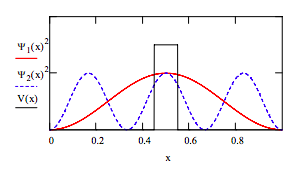
\(\newcommand{\avec}{\mathbf a}\) \(\newcommand{\bvec}{\mathbf b}\) \(\newcommand{\cvec}{\mathbf c}\) \(\newcommand{\dvec}{\mathbf d}\) \(\newcommand{\dtil}{\widetilde{\mathbf d}}\) \(\newcommand{\evec}{\mathbf e}\) \(\newcommand{\fvec}{\mathbf f}\) \(\newcommand{\nvec}{\mathbf n}\) \(\newcommand{\pvec}{\mathbf p}\) \(\newcommand{\qvec}{\mathbf q}\) \(\newcommand{\svec}{\mathbf s}\) \(\newcommand{\tvec}{\mathbf t}\) \(\newcommand{\uvec}{\mathbf u}\) \(\newcommand{\vvec}{\mathbf v}\) \(\newcommand{\wvec}{\mathbf w}\) \(\newcommand{\xvec}{\mathbf x}\) \(\newcommand{\yvec}{\mathbf y}\) \(\newcommand{\zvec}{\mathbf z}\) \(\newcommand{\rvec}{\mathbf r}\) \(\newcommand{\mvec}{\mathbf m}\) \(\newcommand{\zerovec}{\mathbf 0}\) \(\newcommand{\onevec}{\mathbf 1}\) \(\newcommand{\real}{\mathbb R}\) \(\newcommand{\twovec}[2]{\left[\begin{array}{r}#1 \\ #2 \end{array}\right]}\) \(\newcommand{\ctwovec}[2]{\left[\begin{array}{c}#1 \\ #2 \end{array}\right]}\) \(\newcommand{\threevec}[3]{\left[\begin{array}{r}#1 \\ #2 \\ #3 \end{array}\right]}\) \(\newcommand{\cthreevec}[3]{\left[\begin{array}{c}#1 \\ #2 \\ #3 \end{array}\right]}\) \(\newcommand{\fourvec}[4]{\left[\begin{array}{r}#1 \\ #2 \\ #3 \\ #4 \end{array}\right]}\) \(\newcommand{\cfourvec}[4]{\left[\begin{array}{c}#1 \\ #2 \\ #3 \\ #4 \end{array}\right]}\) \(\newcommand{\fivevec}[5]{\left[\begin{array}{r}#1 \\ #2 \\ #3 \\ #4 \\ #5 \\ \end{array}\right]}\) \(\newcommand{\cfivevec}[5]{\left[\begin{array}{c}#1 \\ #2 \\ #3 \\ #4 \\ #5 \\ \end{array}\right]}\) \(\newcommand{\mattwo}[4]{\left[\begin{array}{rr}#1 \amp #2 \\ #3 \amp #4 \\ \end{array}\right]}\) \(\newcommand{\laspan}[1]{\text{Span}\{#1\}}\) \(\newcommand{\bcal}{\cal B}\) \(\newcommand{\ccal}{\cal C}\) \(\newcommand{\scal}{\cal S}\) \(\newcommand{\wcal}{\cal W}\) \(\newcommand{\ecal}{\cal E}\) \(\newcommand{\coords}[2]{\left\{#1\right\}_{#2}}\) \(\newcommand{\gray}[1]{\color{gray}{#1}}\) \(\newcommand{\lgray}[1]{\color{lightgray}{#1}}\) \(\newcommand{\rank}{\operatorname{rank}}\) \(\newcommand{\row}{\text{Row}}\) \(\newcommand{\col}{\text{Col}}\) \(\renewcommand{\row}{\text{Row}}\) \(\newcommand{\nul}{\text{Nul}}\) \(\newcommand{\var}{\text{Var}}\) \(\newcommand{\corr}{\text{corr}}\) \(\newcommand{\len}[1]{\left|#1\right|}\) \(\newcommand{\bbar}{\overline{\bvec}}\) \(\newcommand{\bhat}{\widehat{\bvec}}\) \(\newcommand{\bperp}{\bvec^\perp}\) \(\newcommand{\xhat}{\widehat{\xvec}}\) \(\newcommand{\vhat}{\widehat{\vvec}}\) \(\newcommand{\uhat}{\widehat{\uvec}}\) \(\newcommand{\what}{\widehat{\wvec}}\) \(\newcommand{\Sighat}{\widehat{\Sigma}}\) \(\newcommand{\lt}{<}\) \(\newcommand{\gt}{>}\) \(\newcommand{\amp}{&}\) \(\definecolor{fillinmathshade}{gray}{0.9}\)\( \psi _{1} (x) = \sqrt{2} \sin{ \pi x}\)
\( \psi _{2} (x) = \sqrt{2} \sin{3 \pi x}\)
\( V(x) = if [(x \geq .45) (x \leq .55), 3,0]\)
Plot trial wavefunctions and potential energy.
Evaluate matrix elements for \(100 E_h\) internal barrier:
\( S_{11} = \int_{0}^{1} \psi _{1} (x)^{2} dx\) \( S_{11} = 1\)
\( S_{12} = \int_{0}^{1} \psi _{1} (x) \psi _{2} (x) dx\) \( S_{12} = 0\)
\( S_{22} = \int_{0}^{1} \psi _{2} (x)^{2} dx\) \( S_{22} = 1\)
\[ \begin{align} H_{11} &= \int_{0}^{1} \psi _{1} (x) (- \dfrac{1}{2}) \dfrac{d^{2}}{dx^{2}} \psi _{1} (x) dx + \int_{.45}^{.55} \psi _{1} (x)~100~ \psi _{1} (x) dx\\[4pt] & \approx 24.7711\end{align} \nonumber \]
\[\begin{align} H_{12} &= \int_{0}^{1} \psi _{1} (x) (- \dfrac{1}{2}) \dfrac{d^{2}}{dx^{2}} \psi _{2} (x) dx + \int_{.45}^{.55} \psi _{1} (x)~100~ \psi _{2} (x) dx \\[4pt] & \approx -19.1912\end{align} \nonumber \]
\[\begin{align} H_{22} &= \int_{0}^{1} \psi _{2} (x) (- \dfrac{1}{2}) \dfrac{d^{2}}{dx^{2}} \psi _{2} (x) dx + \int_{.45}^{.55} \psi _{2} (x)~100~ \psi _{2} (x) dx \\[4pt] &\approx 62.9972 \end{align} \nonumber \]
Solve the secular equations and normalization constraint for the energy and coefficients.
Seed values for energy and coefficient: E = 5 c1 = .5 c2 = .5
Given
\( (H_{11} - E S_{11})c_{1} + (H_{12} - E S_{12})c_{2} = 0\)
\( (H_{12} - E S_{12})c_{1} + (H_{22} - E S_{22})c_{2} = 0\)
\( c_{1}^{2} S_{11} + 2 c_{1} c_{2} S_{12} + c_{2}^{2} S_{22} = 1\)
\({\begin{pmatrix}
E \\
c_{1} \\
c_{2}
\end{pmatrix}} = Find(E, c_{1}, c_{2})\)
\({\begin{pmatrix}
E \\
c_{1} \\
c_{2}
\end{pmatrix}} = {\begin{pmatrix} 16.7989 \\
0.9235\\
0.3836
\end{pmatrix}}\)
Plot variational results:
\( \Phi (x) = c_{1} \Phi _{1} (x) + c_{2} \psi_{2} (x)\)
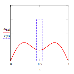
Calculate the probability the particle is in the barrier:
\( \int_{0.45}^{0.55} \Phi (x)^{2} dx = 0.0605\)
Calculate potential and kinetic energy:
\( V = 100 \int_{0.45}^{0.55} \Phi (x)^{2} dx\) \( V = 6.0541\)
\( T = E - V\)
\( T = 10.7448\)