8.75: Qubit Quantum Mechanics

In this document I reproduce most of the results presented in Professor Galvezʹs paper using the Mathcad programming environment.

State Vector

\[ \begin{matrix} \text{Photon moving horizontally:} & \text{x} = \begin{pmatrix} 1 \\ 0 \end{pmatrix} & \text{Photon moving vertically:} & \text{y} = \begin{pmatrix} 0 \\ 1 \end{pmatrix} & \text{Null vector:} & \text{n} = \begin{pmatrix} 0 \\ 0 \end{pmatrix} \\ \text{Horizontal polarization:} & \text{h} = \begin{pmatrix} 1 \\ 0 \end{pmatrix} & \text{Vertical polarization:} & \text{v} = \begin{pmatrix} 0 \\ 1 \end{pmatrix} & \text{Diagonal polarization:} & \text{d} = \begin{pmatrix} \frac{1}{ \sqrt{2}} \\ \frac{1}{ \sqrt{2}} \end{pmatrix} \end{matrix} \nonumber \]

Single mode operators:

Projection operators for motion in the x- and y-directions:

\[ \begin{matrix} \text{X} = \begin{pmatrix} 1 & 0 \\ 0 & 0 \end{pmatrix} & \text{Y} = \begin{pmatrix} 0 & 0 \\ 0 & 1 \end{pmatrix} \end{matrix} \nonumber \]

Operator for polarizing film oriented at an angle of θ to the horizontal.

\[ \Theta_{ \text{op}} ( \theta ) = \begin{pmatrix} \cos \theta \\ \sin \theta \end{pmatrix} \begin{pmatrix} \cos \theta & \sin \theta \end{pmatrix} \rightarrow \begin{pmatrix} \cos \theta^2 & \cos \theta \sin \theta \\ \cos \theta \sin \theta & \sin \theta^2 \end{pmatrix} \nonumber \]

Beam splitter:

\[ \text{BS} = \begin{pmatrix} \frac{1}{ \sqrt{2}} & \frac{i}{ \sqrt{2}} \\ \frac{i}{ \sqrt{2}} & \frac{1}{ \sqrt{2}} \end{pmatrix} \nonumber \]

Mirror:

\[ \text{M} = \begin{pmatrix} 0 & 1 \\ 1 & 0 \end{pmatrix} \nonumber \]

Phase shift:

\[ \text{A}( \delta ) = \begin{pmatrix} e^{i \delta} & 0 \\ 0 & 1 \end{pmatrix} \nonumber \]

Half and quarter wave plate:

\[ \begin{matrix} \text{W}_2 = \begin{pmatrix} 1 & 0 \\ 0 & -1 \end{pmatrix} & \text{W}_4 = \begin{pmatrix} 1 & 0 \\ 0 & -i \end{pmatrix} \end{matrix} \nonumber \]

Identity:

\[ \text{I} = \begin{pmatrix} 1 & 0 \\ 0 & 1 \end{pmatrix} \nonumber \]

Rotated half wave plate:

\[ \begin{matrix} \text{W}_2 ( \theta) = \begin{pmatrix} \cos (2 \theta) & \sin (2 \theta) \\ \sin (2 \theta) & - \cos (2 \theta) \end{pmatrix} & \text{W} ( \theta) = \begin{pmatrix} \cos (2 \theta) & \sin (2 \theta) & 0 & 0 \\ \sin (2 \theta) & - \cos (2 \theta) & 0 & 0 \\ 0 & 0 & 0 & 0 \\ 0 & 0 & 0 & -1 \end{pmatrix} \end{matrix} \nonumber \]

Mach-Zehnder interferometer:

\[ \text{MZ} ( \delta) = \text{BS A} ( \delta) \text{M BS} \nonumber \]

Two mode states and operators:

Single-photon direction of propagation and polarization states:

\[ \begin{matrix} \text{xh} = \begin{pmatrix} 1 \\ 0 \\ 0 \\ 0 \end{pmatrix} & \text{xv} = \begin{pmatrix} 0 \\ 1 \\ 0 \\ 0 \end{pmatrix} & \text{yh} = \begin{pmatrix} 0 \\ 0 \\ 1 \\ 0 \end{pmatrix} & \text{yv} = \begin{pmatrix} 0 \\ 0 \\ 0 \\ 1 \end{pmatrix} \end{matrix} \nonumber \]

Two-photon direction of propagation states.

\[ \begin{matrix} \text{xx} = \begin{pmatrix} 1 \\ 0 \\ 0 \\ 0 \end{pmatrix} & \text{xy} = \begin{pmatrix} 0 \\ 1 \\ 0 \\ 0 \end{pmatrix} & \text{yx} = \begin{pmatrix} 0 \\ 0 \\ 1 \\ 0 \end{pmatrix} & \text{yy} = \begin{pmatrix} 0 \\ 0 \\ 0 \\ 1 \end{pmatrix} \end{matrix} \nonumber \]

Two-photon polarization states:

\[ \begin{matrix} \text{hh} = \begin{pmatrix} 1 \\ 0 \\ 0 \\ 0 \end{pmatrix} & \text{hv} = \begin{pmatrix} 0 \\ 1 \\ 0 \\ 0 \end{pmatrix} & \text{vh} = \begin{pmatrix} 0 \\ 0 \\ 1 \\ 0 \end{pmatrix} & \text{vv} = \begin{pmatrix} 0 \\ 0 \\ 0 \\ 1 \end{pmatrix} \end{matrix} \nonumber \]

Polarizing beam splitter which transmits horizontally polarized photons and reflects vertically polarized photons.

\[ \begin{matrix} \text{PBS} = \text{xh xh}^T + \text{yv xv}^T + \text{yh yh}^T + \text{xv yv}^T & \text{PBS} = \begin{pmatrix} 1 & 0 & 0 & 0 \\ 0 & 0 & 0 & 1 \\ 0 & 0 & 1 & 0 \\ 0 & 1 & 0 & 0 \end{pmatrix} \end{matrix} \nonumber \]

Polarization M-Z interferometer:

\[ \text{MZp} ( \delta) = \text{PBS kronecker} ( \text{A} ( \delta), \text{ I}) \text{kronecker(M, I) PBS} \nonumber \]

Kronecker is Mathcadʹs command for tensor multiplication of square matrices.

Mach‐Zehnder interferometer for direction of propagation and polarization, which places a rotatable half‐wave plate in the upper path.

\[ \text{MZ}_{ \text{dp}} ( \theta, \delta) = \text{kronecker (BS, I) kronecker(A (} \delta) \text{ ,I) W (} \theta \text{) kronecker (M, I) kronecker (BS, I)} \nonumber \]

Mach-Zehnder two-photon direction-of-propagation interferometer.

\[ \begin{matrix} \text{BSBS = kronecker(BS, BS)} & \text{MM = kronecker(M, M)} & \text{AA(} \delta \text{) = kronecker(A(} \delta \text{), A(} \delta)) \\ ~ & \text{MZ}_{ \text{dd}} ( \delta) = \text{BSBS AA} ( \delta) \text{MM BSBS} \end{matrix} \nonumber \]

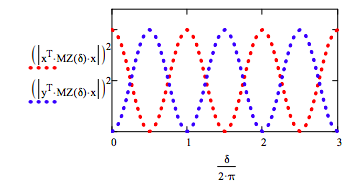
Confirm the results in Figure 2 for the Mach-Zehnder interferometer:

\[ \delta = 0, .125 \pi ... 6 \pi \nonumber \]

Demonstrate that a superposition is formed after the first beam splitter.

\[ \begin{matrix} \text{BS x} = \begin{pmatrix} 0.707 \\ 0.707i \end{pmatrix} & \frac{1}{ \sqrt{2}} \text{(x + iy)} = \begin{pmatrix} 0.707 \\ 0.707i \end{pmatrix} \end{matrix} \nonumber \]

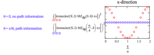
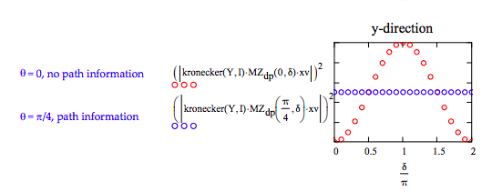
Confirmation that path information destroys interference.

\[ \delta = 0, .1 \pi .. 2 \pi \nonumber \]

Erasure of path information restores interference. Erasers for the x- and y-directions place diagonal polarizers in those directions after the interferometer.

\[ \begin{matrix} \text{E}_{ \text{x}} = \begin{pmatrix} \frac{1}{2} & \frac{1}{2} & 0 & 0 \\ \frac{1}{2} & \frac{1}{2} & 0 & 0 \\ 0 & 0 & 1 & 0 \\ 0 & 0 & 0 & 1 \end{pmatrix} & \text{E}_{ \text{y}} = \begin{pmatrix} 1 & 0 & 0 & 0 \\ 0 & 1 & 0 & 0 \\ 0 & 0 & \frac{1}{2} & \frac{1}{2} \\ 0 & 0 & \frac{1}{2} & \frac{1}{2} \end{pmatrix} \end{matrix} \nonumber \]

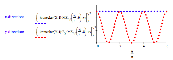
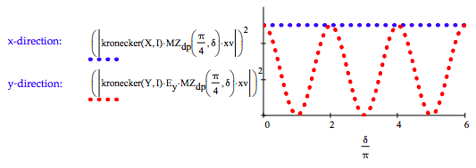
The x-direction has an erase and the y-direction does not.

\[ \delta = 0, .1 \pi .. 6 \pi \nonumber \]

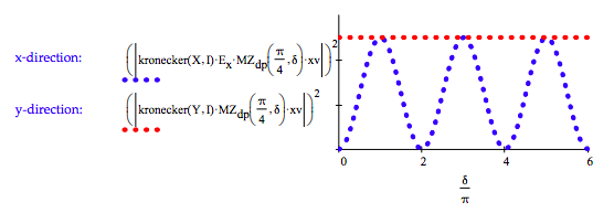
The y-direction has an eraser and the x-direction does not.

For the MZ polarization interferometer diagonally polarized light enters in the x-direction, |xd>. Tensor vector multiplication is awkward in Mathcad as shown below.

\[ \begin{matrix} \Psi_{ \text{in}} = \frac{1}{ \sqrt{2}} \begin{pmatrix} 1 \\ 1 \\ 0 \\ 0 \end{pmatrix} & \text{submatrix(kronecker(augment(x, n), augment(d, n)), 1, 4, 1, 1)} = \begin{pmatrix} 0.707 \\ 0.707 \\ 0 \\ 0 \end{pmatrix} \end{matrix} \nonumber \]

No light, however, exits in the x-direction. It exits in the y-direction showing no interference effects.

\[ \delta = 0, .2 \pi ... \pi \nonumber \]

\[ \begin{matrix} \text{x-direction:} & \text{y-direction:} \\ \left( \left| \text{kronecker(X, I) MZ}_p ( \delta) \Psi_{ \text{in}} \right| \right)^2 = & \left( \left| \text{kronecker(Y, I) MZ)}_p ( \delta) \Psi_{ \text{in}} \right| \right)^2 = \\ \begin{array}{|r|} \hline \\ 0 \\ \hline \\ 0 \\ \hline \\ 0 \\ \hline \\ 0 \\ \hline \\ 0 \\ \hline \\ 0 \\ \hline \end{array} & \begin{array}{|r|} \hline \\ 1 \\ \hline \\ 1 \\ \hline \\ 1 \\ \hline \\ 1 \\ \hline \\ 1 \\ \hline \\ 1 \\ \hline \end{array} \end{matrix} \nonumber \]

Placement of a D polarizer in the y-direction output erases distinguishing information and interference appears.

\[ \delta = 0, .1 \pi .. 6 \pi \nonumber \]

Calculation of exit probabilities for two photons in direction-of-propagation modes:

\[ \begin{matrix} \text{P}_{ \text{xx}} ( \delta) = \left( \left| \text{xx}^T \text{MZ}_{ \text{dd}} ( \delta) \text{xx} \right| \right)^2 & \text{P}_{ \text{xy}} ( \delta) = \left[ \left| \frac{1}{ \sqrt{2}} ( \text{xy + yx})^T \text{MZ}_{ \text{dd}} ( \delta) \text{xx} \right| \right] \\ \text{P}_{ \text{yy}} ( \delta) = \left( \left| \text{yy}^T \text{MZ}_{ \text{dd}} ( \delta) \text{xx} \right| \right)^2 & \text{Tot} ( \delta) = \text{P}_{ \text{xx}} ( \delta) + \text{P}_{ \text{xy}} ( \delta) + \text{P}_{ \text{yy}} ( \delta) \end{matrix} \nonumber \]

Reproduction of Figure 5b with the addition of P_yy.

\[ \delta = 0, .07 \pi .. 6 \pi \nonumber \]

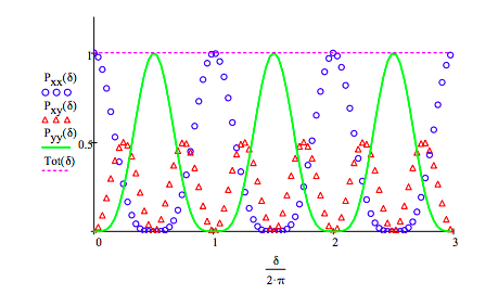
ʺThe striking result is that the (P_xy) interference pattern has twice the frequency of the single‐photon interference pattern. Nonclassical interference shows new quantum aspects: two photons acting as a single quantum object (a biphoton).ʺ

Hong-Ou-Mandel interference (right column, page 516):

\[ \begin{matrix} \text{BSBS} \frac{1}{ \sqrt{2}} \text{(xy + yx)} = \begin{pmatrix} 0.707i \\ 0 \\ 0 \\ 0.707i \end{pmatrix} & \frac{i}{ \sqrt{2}} \text{(xx + yy)} = \begin{pmatrix} 0.707i \\ 0 \\ 0 \\ 0.707i \end{pmatrix} \end{matrix} \nonumber \]

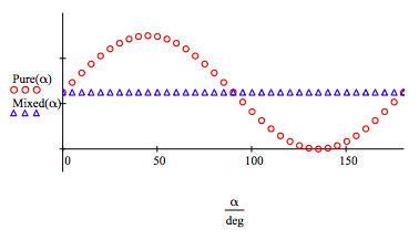
Section III.D deals with distinguishing between pure and mixed states experimentally. The pure state and it density matrix are given below.

\[ \begin{matrix} \Psi_{ \text{pure}} = \frac{1}{ \sqrt{2}} \text{(hh + vv)} & \Psi_{ \text{pure}} = \begin{pmatrix} 0.707 \\ 0 \\ 0 \\ 0.707 \end{pmatrix} & \Psi_{ \text{pure}} \Psi_{ \text{pure}}^T = \begin{pmatrix} 0.5 & 0 & 0 & 0.5 \\ 0 & 0 & 0 & 0 \\ 0 & 0 & 0 & 0 \\ 0.5 & 0 & 0 & 0.5 \end{pmatrix} \end{matrix} \nonumber \]

The density matrix for the mixed state is calculated as follows.

\[ \frac{1}{2} \text{hh hh}^T + \frac{1}{2} \text{vv vv}^T = \begin{pmatrix} 0.5 & 0 & 0 & 0 \\ 0 & 0 & 0 & 0 \\ 0 & 0 & 0 & 0 \\ 0 & 0 & 0 & 0.5 \end{pmatrix} \nonumber \]

The following calculations and their graphical representation are in complete agreement with section III.D

\[ \begin{matrix} \text{Pure}( \alpha) = \text{tr} \left[ \frac{1}{2} \begin{pmatrix} 1 & 0 & 0 & 1 \\ 0 & 0 & 0 & 0 \\ 0 & 0 & 0 & 0 \\ 1 & 0 & 0 & 1 \end{pmatrix} \frac{1}{2} \left[ \begin{pmatrix} \cos \alpha \\ \cos \alpha \\ \sin \alpha \\ \sin \alpha \end{pmatrix} \begin{pmatrix} \cos \alpha \\ \cos \alpha \\ \sin \alpha \\ sin \alpha \end{pmatrix}^T \right] \right] \text{simplify} \rightarrow \frac{ \sin (2 \alpha)}{4} + \frac{1}{4} \end{matrix} \nonumber \]

\[ \begin{matrix} \text{Mixed}( \alpha) = \text{tr} \left[ \frac{1}{2} \begin{pmatrix} 1 & 0 & 0 & 1 \\ 0 & 0 & 0 & 0 \\ 0 & 0 & 0 & 0 \\ 1 & 0 & 0 & 1 \end{pmatrix} \frac{1}{2} \left[ \begin{pmatrix} \cos \alpha \\ \cos \alpha \\ \sin \alpha \\ \sin \alpha \end{pmatrix} \begin{pmatrix} \cos \alpha \\ \cos \alpha \\ \sin \alpha \\ sin \alpha \end{pmatrix}^T \right] \right] \text{simplify} \rightarrow \frac{1}{4} \end{matrix} \nonumber \]

Reproduce Figure 6 results.

\[ \alpha = 0 \text{deg},~ 5 \text{deg} .. 180 \text{deg} \nonumber \]

The following calculation are in agreement with the math in the final paragraph of the section IV.D.

\[ \begin{matrix} \text{kronecker} \left( \text{W}_2 (0),~ \text{I} \right) \Psi_{ \text{pure}} = \begin{pmatrix} 0.707 \\ 0 \\ 0 \\ -0.707 \end{pmatrix} & \begin{pmatrix} 0.707 \\ 0 \\ 0 \\ -0.707 \end{pmatrix} \begin{pmatrix} 0.707 \\ 0 \\ 0 \\ -0.707 \end{pmatrix}^T = \begin{pmatrix} 0.5 & 0 & 0 & -0.5 \\ 0 & 0 & 0 & 0 \\ 0 & 0 & 0 & 0 \\ -0.5 & 0 & 0 & 0.5 \end{pmatrix} \end{matrix} \nonumber \]

\[ \begin{matrix} \text{kronecker} \left( \text{W}_2 (0),~ \text{I}} \right) \Psi_{ \text{pure}} \Psi_{ \text{pure}}^T \text{kronecker} \left( \text{W}_2 (0),~ \text{I} \right)^T = \begin{pmatrix} 0.5 & 0 & 0 & -0.5 \\ 0 & 0 & 0 & 0 \\ 0 & 0 & 0 & 0 \\ -0.5 & 0 & 0 & 0.5 \end{pmatrix} \\ \text{Pure} ( \alpha) = \text{tr} \left[ \frac{1}{2} \begin{pmatrix} 1 & 0 & 0 & -1 \\ 0 & 0 & 0 & 0 \\ 0 & 0 & 0 & 0 \\ -1 & 0 & 0 & 1 \end{pmatrix} \frac{1}{2} \left[ \begin{pmatrix} \cos \alpha \\ \cos \alpha \\ \sin \alpha \\ \sin \alpha \end{pmatrix} \begin{pmatrix} \cos \alpha \\ \cos \alpha \\ \sin \alpha \\ \sin \alpha \end{pmatrix}^T \right] \right] \text{simplify} \rightarrow \frac{1}{4} - \frac{ \sin (2 \alpha)}{4} \end{matrix} \nonumber \]

The paper shows this as \( \frac{[1- \sin \alpha}{4}\) which I am confident is a typographical error.