8.50: EPR Analysis for a Composite Singlet Spin System - Short Version

A spin-1/2 pair is prepared in an entangled singlet state and the individual particles travel in opposite directions on the y-axis to a pair of Stern-Gerlach detectors which are set up to measure spin in the x-z plane. Particle 1's spin is measured along the z-axis, and particle 2's spin is measured at an angle θ with respect to the z-axis.

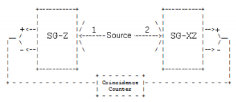
For the singlet state the arrows below indicate the spin orientation for any direction in the x-z plane.

\[ | \Psi \rangle = \frac{1}{ \sqrt{2}} \left[ | \uparrow \rangle_1 | \downarrow \rangle_2 - | \downarrow \rangle_1 | \uparrow \rangle_2 \right] = \frac{1}{ \sqrt{2}} \left[ \begin{pmatrix} \cos \left( \frac{ \theta}{2} \right) \\ \sin \left( \frac{ \theta}{2} \right) \end{pmatrix}_1 \otimes \begin{pmatrix} - \sin \left( \frac{ \theta}{2} \right) \\ \cos \left( \frac{ \theta}{2} \right) \end{pmatrix}_2 - \begin{pmatrix} - \sin \left( \frac{ \theta}{2} \right) \\ \cos \left( \frac{ \theta}{2} \right) \end{pmatrix}_1 \otimes \begin{pmatrix} \cos \left( \frac{ \theta}{2} \right) \\ \sin \left( \frac{ \theta}{2} \right) \end{pmatrix}_2 \right] = \frac{1}{ \sqrt{2}} \begin{pmatrix} 0 \\ 1 \\ -1 \\ 0 \end{pmatrix} \nonumber \]

The single particle spin operator in the x-z plane is constructed from the Pauli spin operators in the x- and z-directions. φ is the angle of orientation of the measurement magnet with the z-axis.

\[ \begin{matrix} \sigma_z = \begin{pmatrix} 1 & 0 \\ 0 & -1 \end{pmatrix} & \sigma_x = \begin{pmatrix} 0 & 1 \\ 1 & 0 \end{pmatrix} & S( \theta) = \cos ( \theta) \sigma_z + \sin ( \theta) \sigma_x \rightarrow \begin{pmatrix} \cos ( \theta) & \sin ( \theta) \\ \sin ( \theta) & - \cos ( \theta) \end{pmatrix} & S(0) = \begin{pmatrix} 1 & 0 \\ 0 & -1 \end{pmatrix} \end{matrix} \nonumber \]

Tensor multiplication of S(0) and S(φ) creates a joint spin measurement operator.

\[ \begin{pmatrix} 1 & 0 \\ 0 & -1 \end{pmatrix} \otimes \begin{pmatrix} \cos \theta & \sin \theta \\ \sin \theta & - \cos \theta \end{pmatrix} = \begin{pmatrix} \cos \theta & \sin \theta & 0 & 0 \\ \sin \theta & - \cos \theta & 0 & 0 \\ 0 & 0 & - \cos \theta & - \sin \theta \\ 0 & 0 - \sin \theta & \cos \theta \end{pmatrix} \frac{1}{ \sqrt{2}} \begin{pmatrix} 0 \\ 1 \\ -1 \\ 0 \end{pmatrix} \nonumber \]

The expectation value as a function of the measurement angle of particle 2 is calculated and the result displayed graphically.

\[ E( \theta) = \frac{1}{ \sqrt{2}} \begin{pmatrix} 0 & 1 & -1 & 0 \end{pmatrix} \begin{pmatrix} \cos \theta & \sin \theta & 0 & 0 \\ \sin \theta & - \cos \theta & 0 & 0 \\ 0 & 0 & - \cos \theta & - \sin \theta \\ 0 & 0 - \sin \theta & \cos \theta \end{pmatrix} \frac{1}{ \sqrt{2}} \begin{pmatrix} 0 \\ 1 \\ -1 \\ 0 \end{pmatrix} \rightarrow - \cos \theta \nonumber \]

For θ = 0⁰ there is perfect anti-correlation; for θ = 180⁰ perfect correlation; for θ = 90⁰ no correlation. A correlation function based on a local-realistic, hidden-variable model (see Fig. 11.2 and related text in A. I. M. Rae's Quantum Mechanics, 2nd Ed.) and the quantum mechanical correlation function, E(θ), are compared on the graph below. Quantum theory and local realism disagree at all angles except 0, 90 and 180 degrees.

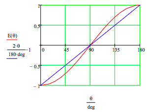
This example illustrates Bell's theorem: no local hidden-variable theory can reproduce all the predictions of quantum mechanics for entangled composite systems. As the quantum predictions are confirmed experimentally, the local hidden-variable approach to reality must be abandoned.