
8.45: Yet Another Assault on Local Realism - A Matrix/Tensor Algebra Approach
- Page ID
- 144089

The purpose of this tutorial is to review Nick Herbertʹs ʺsimple proof of Bellʹs theoremʺ as presented in Chapter 12 of Quantum Reality using matrix and tensor algebra.
A two‐stage atomic cascade emits entangled photons (A and B) in opposite directions with the same circular polarization according to the observers in their path.
\[ | \Psi \rangle = \frac{1}{ \sqrt{2}} \left[ | L \rangle_A |L \rangle_B + |R \rangle_A |R \rangle_B \right] \nonumber \]
The experiment involves the measurement of photon polarization states in the vertical/horizontal measurement basis, and allows that the polarization analyzers (PAs) can be oriented at different angles a and b. (The figure below is similar to the one on page 125 of Jim Baggottʹs The Meaning of Quantum Theory, which provides a thorough analysis of correlated two‐photon experiments.)
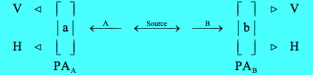
To dramatize the quantum weirdness of this EPR experiment, Herbert places PAA on earth and PAB on Betelgeuse, 540 light years away. The source is a space ship midway between the PAs.
In the vertical/horizontal measurement basis the initial polarization state is (see Appendix A for a justification),
\[ \begin{matrix} | VV \rangle = \begin{pmatrix} 1 \\ 0 \end{pmatrix} \otimes \begin{pmatrix} 1 \\ 0 \end{pmatrix} = \begin{pmatrix} 1 \\ 0 \\ 0 \\ 0 \end{pmatrix} & | VH \rangle = \begin{pmatrix} 1 \\ 0 \end{pmatrix} \otimes \begin{pmatrix} 0 \\ 1 \end{pmatrix} = \begin{pmatrix} 0 \\ 1 \\ 0 \\ 0 \end{pmatrix} & | HV \rangle = \begin{pmatrix} 0 \\ 1 \end{pmatrix} \otimes \begin{pmatrix} 1 \\ 0 \end{pmatrix} = \begin{pmatrix} 0 \\ 0 \\ 1 \\ 0 \end{pmatrix} & | HH \rangle = \begin{pmatrix} 0 \\ 1 \end{pmatrix} \otimes \begin{pmatrix} 0 \\ 1 \end{pmatrix} = \begin{pmatrix} 0 \\ 0 \\ 0 \\ 1 \end{pmatrix} \end{matrix} \nonumber \]
We now write all states, Ψ and the measurement states, in Mathcad's vector format.
\[ \begin{matrix} \Psi = \frac{1}{ \sqrt{2}} \begin{pmatrix} 1 \\ 0 \\ 0 \\ -1 \end{pmatrix} & | VV \rangle = \begin{pmatrix} 1 \\ 0 \\ 0 \\ 0 \end{pmatrix} & | VH \rangle = \begin{pmatrix} 0 \\ 1 \\ 0 \\ 0 \end{pmatrix} & | HV \rangle = \begin{pmatrix} 0 \\ 0 \\ 1 \\ 0 \end{pmatrix} & | HH \rangle = \begin{pmatrix} 0 \\ 0 \\ 0 \\ 1 \end{pmatrix} \end{matrix} \nonumber \]
Next, the operator representing the rotation of PAA by angle a clockwise and PAB by angle b counter‐clockwise (so that the PAs turn in the same direction) is constructed using matrix tensor multiplication. Kronecker is Mathcadʹs command for tensor matrix multiplication.
\[ \text{RotOp}(a,~b) = \text{kronecker} \begin{bmatrix} \begin{pmatrix} \cos a & - \sin a \\ \sin a & \cos a \end{pmatrix}, ~ \begin{pmatrix} \cos b & \sin b \\ - \sin b & \cos b \end{pmatrix} \end{bmatrix} \nonumber \]
The probability that the detectors will behave the same or differently is calculated as follows.
\[ \begin{pmatrix} P_{same} (a,~b) = \left( VV^T \text{RotOp}(a,~b) \Psi \right)^2 + \left( HH^T \text{RotOp}(a,~b) \Psi \right)^2 \\ P_{diff} (a,~b) = \left( VH^T \text{RotOp}(a,~b) \Psi \right)^2 + \left( HV^T \text{RotOp}(a,~b) \Psi \right)^2 \end{pmatrix} \nonumber \]
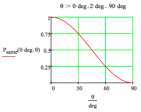
Now we can get on with some actual calculations. The following calculations show that if the PAs are oriented at the same angle they behave the same way 100% of the time. This is called perfect correlation.
\[ \begin{matrix} P_{same} \text{(0 deg, 0 deg)} = 100 \% & P_{same} \text{(30 deg, 30 deg)} = 100 \% & P_{same} \text{(90 deg, 90 deg)} = 100 \% \\ P_{diff} \text{(0 deg, 0 deg)} = 0 \% & P_{diff} \text{(30 deg, 30 deg)} = 0 \% & P_{diff} \text{(90 deg, 90 deg)} = 0 \% \end{matrix} \nonumber \]
These results appear to support the notion that the linear polarization states of the photons are ʺelements of reality.ʺ In other words, they are photon properties that exist independent of observation. However, this position is not supported by further calculation and experimentation.
Perfect anti‐correlation occurs when the relative angle between the PAs is 90 degrees.
\[ \begin{matrix} P_{same} \text{(0 deg, 0 deg)} = 100 \% & P_{diff} \text{(0 deg, 0 deg)} = 0 \% \end{matrix} \nonumber \]
At 45 degrees there is no correlation between the detectors.
\[ \begin{matrix} P_{same} \text{(0 deg, 45 deg)} = 50 \% & P_{diff} \text{(0 deg, 45 deg)} = 50 \% \end{matrix} \nonumber \]
Using 0 degrees for both PAs as the bench mark, Herbertʹs analysis proceeds by moving PAB to 30 degrees and noting that this leads to a 25% (1 in 4) discrepancy between the analyzers.
\[ \begin{matrix} P_{same} \text{(0 deg, 30 deg)} = 75 \% & P_{diff} \text{(0 deg, 30 deg)} = 25 \% \end{matrix} \nonumber \]
If instead PAA had been moved to ‐30 degrees the result is the same, the PAs disagree 25% of the time.
\[ \begin{matrix} P_{same} \text{(-30 deg, 0 deg)} = 75 \% & P_{diff} \text{(-30 deg, 0 deg)} = 25 \% \end{matrix} \nonumber \]
Now the locality principal is invoked. The PAs are spatially separated so that according to conventional intuition, the change in the orientation of PAB has no effect on the results at PAA, and vice versa.
Now Herbert moves PAB back to 30 degrees with the following result.
\[ \begin{matrix} P_{same} \text{(-30 deg, 30 deg)} = 25 \% & P_{diff} \text{(-30 deg, 30 deg)} = 75 \% \end{matrix} \nonumber \]
The angular difference is now 60 degrees, and the PAs disagree 75% of the time. On the basis of local realism one would expect a discrepancy of no more than 50% . If the measurements at the PAs are independent of each other, we should simply be able to add 25% and 25%. A more general version this approach to Bellʹs theorem can be found in the Appendix B.
The experiment was performed by John Clauser and Stuart Freedman at Berkeley in 1972 and confirmed the quantum predictions. The agreement between quantum theory and experiment requires that some element of local realism must be abandoned. The consensus is that nature allows non‐local interactions for entangled systems such as the photons in this example. The results at PAA and PAB (light years apart) are connected by a non‐local interaction. This type of interaction is, in the words of Herbert, ʺunmediated, unmitigated and immediate.ʺ
Many other experiments besides those of Clauser and Freedman (most notably by Aspect and co‐workers) have confirmed quantum mechanical predictions and refuted local realism. Anton Zeilinger described the current situation as follows:
By now, a number of experiments have confirmed quantum predictions to such an extent that a local‐realistic world view can no longer be maintained.
It appears that, certainly at least for entangled quantum systems, it is wrong to assume that the features of the world which we observe, the measurement results, exist prior to and independently of our observation.
Appendix A
In vector notation the left‐ and right‐circular polarization states are expressed as follows:
Left circular polarization:
\[ L = \frac{1}{ \sqrt{2}} \begin{pmatrix} 1 \\ i \end{pmatrix} \nonumber \]
Right circular polarization:
\[ R = \frac{1}{ \sqrt{2}} \begin{pmatrix} 1 \\ -i \end{pmatrix} \nonumber \]
In tensor notation the initial photon state is,
\[ | \Psi \rangle = \frac{1}{ \sqrt{2}} \left[ |L \rangle_A |L \rangle_B + |R \rangle_A |R \rangle_B \right] = \frac{1}{ 2 \sqrt{2}} \left[ \begin{pmatrix} 1 \\ i \end{pmatrix}_A \otimes \begin{pmatrix} 1 \\ i \end{pmatrix}_B + \begin{pmatrix} 1 \\ -i \end{pmatrix}_A \otimes \begin{pmatrix} 1 \\ -i \end{pmatrix}_B \right] = \frac{1}{ 2 \sqrt{2}} \left[ \begin{pmatrix} 1 \\ i \\ i \\ -1 \end{pmatrix} + \begin{pmatrix} 1 \\ -i \\ -i \\ -1 \end{pmatrix} \right] = \frac{1}{ \sqrt{2}} \begin{pmatrix} 1 \\ 0 \\ 0 \\ -1 \end{pmatrix} \nonumber \]
Vertical polarization:
\[ V = \begin{pmatrix} 1 \\ 0 \end{pmatrix} \nonumber \]
Horizontal polarization:
\[ H = \begin{pmatrix} 0 \\ 1 \end{pmatrix} \nonumber \]
It is easy to show that the equivalent vertical/horizontal polarization state is,
\[ | \Psi \rangle = \frac{1}{ \sqrt{2}} \left[ |V \rangle_A |V \rangle_B + |H \rangle_A |H \rangle_B \right] = \frac{1}{ 2 \sqrt{2}} \left[ \begin{pmatrix} 1 \\ 0 \end{pmatrix}_A \otimes \begin{pmatrix} 1 \\ 0 \end{pmatrix}_B + \begin{pmatrix} 0 \\ 1 \end{pmatrix}_A \otimes \begin{pmatrix} 0 \\ 1 \end{pmatrix}_B \right] = \frac{1}{ 2 \sqrt{2}} \left[ \begin{pmatrix} 1 \\ 0 \\ 0 \\ 0 \end{pmatrix} - \begin{pmatrix} 0 \\ 0 \\ 0 \\ 1 \end{pmatrix} \right] = \frac{1}{ \sqrt{2}} \begin{pmatrix} 1 \\ 0 \\ 0 \\ -1 \end{pmatrix} \nonumber \]
Naturally there are other ways to do this. The most direct would be to write |L> and |R> as superpositions of |V> and |H>, and substitute them into the initial state involving the circular polarization states.
\[ \psi = \frac{1}{ \sqrt{2}} (L_A L_B + R_A R_B ) ~ \begin{array}{|l} \text{substitute, } L_A = \frac{1}{ \sqrt{2}} (V_A + iH_A) \\ \text{substitute, } L_B = \frac{1}{ \sqrt{2}} (V_B + iH_B) \\ \text{substitute, } L_A = \frac{1}{ \sqrt{2}} (V_A + iH_A) \\ \text{substitute, } L_A = \frac{1}{ \sqrt{2}} (V_A + iH_A) \\ \text{simplify} \end{array} \rightarrow \psi = \frac{ \sqrt{2} V_A V_B}{2} - \frac{ \sqrt{2} H_A H_B}{2} \nonumber \]
Figure 12.4 on page 223 in Herbert's Quantum Reality is reproduced.
Appendix B
It is not difficult to derive the following Bell inequality based on local realism involving three sets of polarization measurement angles for the experiment described above. See The Meaning of Quantum Theory by Jim Baggott, pages 133‐135.
\[ P_{diff} (a,~ b) + P_{diff} (a,~b) \geq P_{diff} (a,~c) \nonumber \]
Below it is shown that the inequality is violated for 0, 22.5 and 45 degrees, as well as for 0, 30 and 60 degrees.
\[ \begin{matrix} P_{diff} \text{(0 deg, 22.5 deg)} + P_{diff} \text{(22.5 deg, 45 deg)} = 0.293 & P_{diff} \text{(0 deg, 45 deg)} = 0.5 \\ P_{diff} \text{(0 deg, 30 deg)} + P_{diff} \text{(30 deg, 60 deg)} = 0.5 & P_{diff} \text{(0 deg, 60 deg)} = 0.75 \end{matrix} \nonumber \]
The Bell inequality is also violated for other sets of angles. However, it is not violated for 0, 45 and 90 degrees.
\[ \begin{matrix} P_{diff} \text{(0 deg, 45 deg)} + P_{diff} \text{(45 deg, 90 deg)} = 1 & P_{diff} \text{(0 deg, 90 deg)} = 1 \end{matrix} \nonumber \]
On page 135 Baggott summarizes the significance of Bellʹs inequality.
The most important assumption ... made in the reasoning which led to this inequality was that of ... the local reality of the photons. It is therefore an inequality that is quite independent of the nature of any local hidden variable theory that we could possibly devise. The conclusion is inescapable, quantum theory is incompatible with any local hidden variable theory and hence local reality.
On page 131 he writes that after Bellʹs work,
Questions about local hidden variables immediately changed character. From being rather academic questions about philosophy they became questions of profound importance for quantum theory. The choice between quantum theory and local hidden variable theories was no longer a question of taste, it was a matter of correctness.
This obviously suggests that clever experimentalist might be able to decide which view of reality is correct. To date experimental results have been consistent with the quantum mechanical predictions.