
5.18: Another Look at the Double-Slit Experiment
- Page ID
- 150543

\( \newcommand{\vecs}[1]{\overset { \scriptstyle \rightharpoonup} {\mathbf{#1}} } \)
\( \newcommand{\vecd}[1]{\overset{-\!-\!\rightharpoonup}{\vphantom{a}\smash {#1}}} \)
\( \newcommand{\id}{\mathrm{id}}\) \( \newcommand{\Span}{\mathrm{span}}\)
( \newcommand{\kernel}{\mathrm{null}\,}\) \( \newcommand{\range}{\mathrm{range}\,}\)
\( \newcommand{\RealPart}{\mathrm{Re}}\) \( \newcommand{\ImaginaryPart}{\mathrm{Im}}\)
\( \newcommand{\Argument}{\mathrm{Arg}}\) \( \newcommand{\norm}[1]{\| #1 \|}\)
\( \newcommand{\inner}[2]{\langle #1, #2 \rangle}\)
\( \newcommand{\Span}{\mathrm{span}}\)
\( \newcommand{\id}{\mathrm{id}}\)
\( \newcommand{\Span}{\mathrm{span}}\)
\( \newcommand{\kernel}{\mathrm{null}\,}\)
\( \newcommand{\range}{\mathrm{range}\,}\)
\( \newcommand{\RealPart}{\mathrm{Re}}\)
\( \newcommand{\ImaginaryPart}{\mathrm{Im}}\)
\( \newcommand{\Argument}{\mathrm{Arg}}\)
\( \newcommand{\norm}[1]{\| #1 \|}\)
\( \newcommand{\inner}[2]{\langle #1, #2 \rangle}\)
\( \newcommand{\Span}{\mathrm{span}}\) \( \newcommand{\AA}{\unicode[.8,0]{x212B}}\)
\( \newcommand{\vectorA}[1]{\vec{#1}} % arrow\)
\( \newcommand{\vectorAt}[1]{\vec{\text{#1}}} % arrow\)
\( \newcommand{\vectorB}[1]{\overset { \scriptstyle \rightharpoonup} {\mathbf{#1}} } \)
\( \newcommand{\vectorC}[1]{\textbf{#1}} \)
\( \newcommand{\vectorD}[1]{\overrightarrow{#1}} \)
\( \newcommand{\vectorDt}[1]{\overrightarrow{\text{#1}}} \)
\( \newcommand{\vectE}[1]{\overset{-\!-\!\rightharpoonup}{\vphantom{a}\smash{\mathbf {#1}}}} \)
\( \newcommand{\vecs}[1]{\overset { \scriptstyle \rightharpoonup} {\mathbf{#1}} } \)
\( \newcommand{\vecd}[1]{\overset{-\!-\!\rightharpoonup}{\vphantom{a}\smash {#1}}} \)
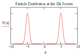
\(\newcommand{\avec}{\mathbf a}\) \(\newcommand{\bvec}{\mathbf b}\) \(\newcommand{\cvec}{\mathbf c}\) \(\newcommand{\dvec}{\mathbf d}\) \(\newcommand{\dtil}{\widetilde{\mathbf d}}\) \(\newcommand{\evec}{\mathbf e}\) \(\newcommand{\fvec}{\mathbf f}\) \(\newcommand{\nvec}{\mathbf n}\) \(\newcommand{\pvec}{\mathbf p}\) \(\newcommand{\qvec}{\mathbf q}\) \(\newcommand{\svec}{\mathbf s}\) \(\newcommand{\tvec}{\mathbf t}\) \(\newcommand{\uvec}{\mathbf u}\) \(\newcommand{\vvec}{\mathbf v}\) \(\newcommand{\wvec}{\mathbf w}\) \(\newcommand{\xvec}{\mathbf x}\) \(\newcommand{\yvec}{\mathbf y}\) \(\newcommand{\zvec}{\mathbf z}\) \(\newcommand{\rvec}{\mathbf r}\) \(\newcommand{\mvec}{\mathbf m}\) \(\newcommand{\zerovec}{\mathbf 0}\) \(\newcommand{\onevec}{\mathbf 1}\) \(\newcommand{\real}{\mathbb R}\) \(\newcommand{\twovec}[2]{\left[\begin{array}{r}#1 \\ #2 \end{array}\right]}\) \(\newcommand{\ctwovec}[2]{\left[\begin{array}{c}#1 \\ #2 \end{array}\right]}\) \(\newcommand{\threevec}[3]{\left[\begin{array}{r}#1 \\ #2 \\ #3 \end{array}\right]}\) \(\newcommand{\cthreevec}[3]{\left[\begin{array}{c}#1 \\ #2 \\ #3 \end{array}\right]}\) \(\newcommand{\fourvec}[4]{\left[\begin{array}{r}#1 \\ #2 \\ #3 \\ #4 \end{array}\right]}\) \(\newcommand{\cfourvec}[4]{\left[\begin{array}{c}#1 \\ #2 \\ #3 \\ #4 \end{array}\right]}\) \(\newcommand{\fivevec}[5]{\left[\begin{array}{r}#1 \\ #2 \\ #3 \\ #4 \\ #5 \\ \end{array}\right]}\) \(\newcommand{\cfivevec}[5]{\left[\begin{array}{c}#1 \\ #2 \\ #3 \\ #4 \\ #5 \\ \end{array}\right]}\) \(\newcommand{\mattwo}[4]{\left[\begin{array}{rr}#1 \amp #2 \\ #3 \amp #4 \\ \end{array}\right]}\) \(\newcommand{\laspan}[1]{\text{Span}\{#1\}}\) \(\newcommand{\bcal}{\cal B}\) \(\newcommand{\ccal}{\cal C}\) \(\newcommand{\scal}{\cal S}\) \(\newcommand{\wcal}{\cal W}\) \(\newcommand{\ecal}{\cal E}\) \(\newcommand{\coords}[2]{\left\{#1\right\}_{#2}}\) \(\newcommand{\gray}[1]{\color{gray}{#1}}\) \(\newcommand{\lgray}[1]{\color{lightgray}{#1}}\) \(\newcommand{\rank}{\operatorname{rank}}\) \(\newcommand{\row}{\text{Row}}\) \(\newcommand{\col}{\text{Col}}\) \(\renewcommand{\row}{\text{Row}}\) \(\newcommand{\nul}{\text{Nul}}\) \(\newcommand{\var}{\text{Var}}\) \(\newcommand{\corr}{\text{corr}}\) \(\newcommand{\len}[1]{\left|#1\right|}\) \(\newcommand{\bbar}{\overline{\bvec}}\) \(\newcommand{\bhat}{\widehat{\bvec}}\) \(\newcommand{\bperp}{\bvec^\perp}\) \(\newcommand{\xhat}{\widehat{\xvec}}\) \(\newcommand{\vhat}{\widehat{\vvec}}\) \(\newcommand{\uhat}{\widehat{\uvec}}\) \(\newcommand{\what}{\widehat{\wvec}}\) \(\newcommand{\Sighat}{\widehat{\Sigma}}\) \(\newcommand{\lt}{<}\) \(\newcommand{\gt}{>}\) \(\newcommand{\amp}{&}\) \(\definecolor{fillinmathshade}{gray}{0.9}\)Illumination of a double-slit screen with a coherent particle beam leads to a Schrödinger "cat state" that can be represented by a linear superposition (unnormalized) of two Gaussian wavepackets. The probability distribution function in coordinate space, |Y(x)|2, at the slit-screen for this "cat state" is shown below.
\[ \begin{matrix} x = -10, ~ -9.99 .. 10 & \Psi (x) = exp \left[ -(x-5)^2 \right] + exp \left[ - (x + 5)^2 \right] & P(x) = \left( \left| \Psi (x) \right| \right)^2 \end{matrix} \nonumber \]
The slits localize the particle in the x-direction which leads to a spread in the x-component of the momentum required by the uncertainty principle, DxDpx > h/4p. The momentum wave function is obtained by a Fourier transform of the coordinate-space wave function.
\[ \Phi (p_x) = \frac{1}{ \sqrt{2 \pi}} \left[ \int_{- \infty}^{ \infty} exp (-i p_x x) \left[ exp \left[ - (x-5)^2 \right] + exp \left[ - (x+5)^2 \right] \right] dx \right] \nonumber \]
Evaluation of the integral yields,
\[ \Phi (p_x ) = \frac{1}{ \sqrt{2}} \left[ exp \left[ \frac{-1}{4} p_x (p_x + 20i) \right] + exp \left[ \frac{-1}{4} p_x (p_x - 20i \right] \right] \nonumber \]
The momentum probability function in the x-direction is |F(px)|2 and simplifies to the expression given below when evaluated.
\[ P(p_x) = 2 exp \left( \frac{-1}{2} p_x^2 \right) \cos (5 p_x )^2 \nonumber \]
This momentum probability function is displayed below.
\[ p_x = -4, -3.99 .. 4 \nonumber \]
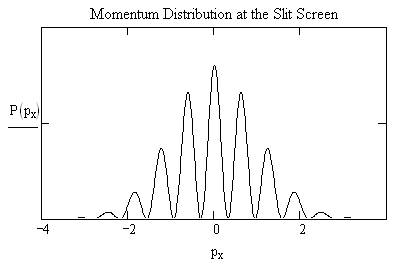
Because the arrival at position x on the detection screen is proportional to px it is also proportional to |F(px)|2. In other words, the particle distribution at the detection screen is determined by the momentum distribution at the slit screen. This means the position measurement at the detection screen is effectively a measurement of the px. Therefore, the particle distribution at the detector screen will have the same shape as shown in the figure above.
In summary, the double-slit experiment clearly reveals the three essential steps in a quantum mechanical experiment:
1. State preparation (interaction of the incident beam with the slit-screen)
2. Measurement of an observable (arrival of scattered beam at the detection screen)
3. Calculation of expected results of the measurement step
*The preparation of this tutorial was stimulated by reading "Quantum interference with slits" by Thomas Marcella which appeared in European Journal of Physics 23, 615-621 (2002). This paper offers a lucid and novel quantum mechanical analysis of a very important experiment.
Additional references:
R. P. Feynman, R. B. Leighton, and M.Sands, The Feynman Lectures on Physics, Volume 3; Addison-Wesley; Reading, 1965, Chapters 1 and 3.
R. P. Feynman, The Character of Physical Law; MIT Press: Cambridge, 1967, Chapter 6.
A. Tonomura, J. Endo, T. Matsuda, T. Kawasaki, and H. Exawa, "Demonstration of single-electron buildup of an interference pattern" Am. J. Phys. 57, 117-120 (1989).
D. Leibfried, T. Pfau, and C. Monroe, "Shadows and Mirrors: Reconstructing Quantum States of Atom Motion" Phys. Today 51(4), 22-28 (1998).
The double-slit experiment with single electrons was recently selected (informally) as physics most beautiful experiment. The following web reference traces the history of double-slit interference experiments from the time of Thomas Young to the present, presenting numerous literature references in the process: http://physicsweb.org/article/world/15/9/1.