
5.8: Is a Two-dimensional Fibonacci Array a Quasilattice?
- Page ID
- 150523

\( \newcommand{\vecs}[1]{\overset { \scriptstyle \rightharpoonup} {\mathbf{#1}} } \)
\( \newcommand{\vecd}[1]{\overset{-\!-\!\rightharpoonup}{\vphantom{a}\smash {#1}}} \)
\( \newcommand{\id}{\mathrm{id}}\) \( \newcommand{\Span}{\mathrm{span}}\)
( \newcommand{\kernel}{\mathrm{null}\,}\) \( \newcommand{\range}{\mathrm{range}\,}\)
\( \newcommand{\RealPart}{\mathrm{Re}}\) \( \newcommand{\ImaginaryPart}{\mathrm{Im}}\)
\( \newcommand{\Argument}{\mathrm{Arg}}\) \( \newcommand{\norm}[1]{\| #1 \|}\)
\( \newcommand{\inner}[2]{\langle #1, #2 \rangle}\)
\( \newcommand{\Span}{\mathrm{span}}\)
\( \newcommand{\id}{\mathrm{id}}\)
\( \newcommand{\Span}{\mathrm{span}}\)
\( \newcommand{\kernel}{\mathrm{null}\,}\)
\( \newcommand{\range}{\mathrm{range}\,}\)
\( \newcommand{\RealPart}{\mathrm{Re}}\)
\( \newcommand{\ImaginaryPart}{\mathrm{Im}}\)
\( \newcommand{\Argument}{\mathrm{Arg}}\)
\( \newcommand{\norm}[1]{\| #1 \|}\)
\( \newcommand{\inner}[2]{\langle #1, #2 \rangle}\)
\( \newcommand{\Span}{\mathrm{span}}\) \( \newcommand{\AA}{\unicode[.8,0]{x212B}}\)
\( \newcommand{\vectorA}[1]{\vec{#1}} % arrow\)
\( \newcommand{\vectorAt}[1]{\vec{\text{#1}}} % arrow\)
\( \newcommand{\vectorB}[1]{\overset { \scriptstyle \rightharpoonup} {\mathbf{#1}} } \)
\( \newcommand{\vectorC}[1]{\textbf{#1}} \)
\( \newcommand{\vectorD}[1]{\overrightarrow{#1}} \)
\( \newcommand{\vectorDt}[1]{\overrightarrow{\text{#1}}} \)
\( \newcommand{\vectE}[1]{\overset{-\!-\!\rightharpoonup}{\vphantom{a}\smash{\mathbf {#1}}}} \)
\( \newcommand{\vecs}[1]{\overset { \scriptstyle \rightharpoonup} {\mathbf{#1}} } \)
\( \newcommand{\vecd}[1]{\overset{-\!-\!\rightharpoonup}{\vphantom{a}\smash {#1}}} \)
\(\newcommand{\avec}{\mathbf a}\) \(\newcommand{\bvec}{\mathbf b}\) \(\newcommand{\cvec}{\mathbf c}\) \(\newcommand{\dvec}{\mathbf d}\) \(\newcommand{\dtil}{\widetilde{\mathbf d}}\) \(\newcommand{\evec}{\mathbf e}\) \(\newcommand{\fvec}{\mathbf f}\) \(\newcommand{\nvec}{\mathbf n}\) \(\newcommand{\pvec}{\mathbf p}\) \(\newcommand{\qvec}{\mathbf q}\) \(\newcommand{\svec}{\mathbf s}\) \(\newcommand{\tvec}{\mathbf t}\) \(\newcommand{\uvec}{\mathbf u}\) \(\newcommand{\vvec}{\mathbf v}\) \(\newcommand{\wvec}{\mathbf w}\) \(\newcommand{\xvec}{\mathbf x}\) \(\newcommand{\yvec}{\mathbf y}\) \(\newcommand{\zvec}{\mathbf z}\) \(\newcommand{\rvec}{\mathbf r}\) \(\newcommand{\mvec}{\mathbf m}\) \(\newcommand{\zerovec}{\mathbf 0}\) \(\newcommand{\onevec}{\mathbf 1}\) \(\newcommand{\real}{\mathbb R}\) \(\newcommand{\twovec}[2]{\left[\begin{array}{r}#1 \\ #2 \end{array}\right]}\) \(\newcommand{\ctwovec}[2]{\left[\begin{array}{c}#1 \\ #2 \end{array}\right]}\) \(\newcommand{\threevec}[3]{\left[\begin{array}{r}#1 \\ #2 \\ #3 \end{array}\right]}\) \(\newcommand{\cthreevec}[3]{\left[\begin{array}{c}#1 \\ #2 \\ #3 \end{array}\right]}\) \(\newcommand{\fourvec}[4]{\left[\begin{array}{r}#1 \\ #2 \\ #3 \\ #4 \end{array}\right]}\) \(\newcommand{\cfourvec}[4]{\left[\begin{array}{c}#1 \\ #2 \\ #3 \\ #4 \end{array}\right]}\) \(\newcommand{\fivevec}[5]{\left[\begin{array}{r}#1 \\ #2 \\ #3 \\ #4 \\ #5 \\ \end{array}\right]}\) \(\newcommand{\cfivevec}[5]{\left[\begin{array}{c}#1 \\ #2 \\ #3 \\ #4 \\ #5 \\ \end{array}\right]}\) \(\newcommand{\mattwo}[4]{\left[\begin{array}{rr}#1 \amp #2 \\ #3 \amp #4 \\ \end{array}\right]}\) \(\newcommand{\laspan}[1]{\text{Span}\{#1\}}\) \(\newcommand{\bcal}{\cal B}\) \(\newcommand{\ccal}{\cal C}\) \(\newcommand{\scal}{\cal S}\) \(\newcommand{\wcal}{\cal W}\) \(\newcommand{\ecal}{\cal E}\) \(\newcommand{\coords}[2]{\left\{#1\right\}_{#2}}\) \(\newcommand{\gray}[1]{\color{gray}{#1}}\) \(\newcommand{\lgray}[1]{\color{lightgray}{#1}}\) \(\newcommand{\rank}{\operatorname{rank}}\) \(\newcommand{\row}{\text{Row}}\) \(\newcommand{\col}{\text{Col}}\) \(\renewcommand{\row}{\text{Row}}\) \(\newcommand{\nul}{\text{Nul}}\) \(\newcommand{\var}{\text{Var}}\) \(\newcommand{\corr}{\text{corr}}\) \(\newcommand{\len}[1]{\left|#1\right|}\) \(\newcommand{\bbar}{\overline{\bvec}}\) \(\newcommand{\bhat}{\widehat{\bvec}}\) \(\newcommand{\bperp}{\bvec^\perp}\) \(\newcommand{\xhat}{\widehat{\xvec}}\) \(\newcommand{\vhat}{\widehat{\vvec}}\) \(\newcommand{\uhat}{\widehat{\uvec}}\) \(\newcommand{\what}{\widehat{\wvec}}\) \(\newcommand{\Sighat}{\widehat{\Sigma}}\) \(\newcommand{\lt}{<}\) \(\newcommand{\gt}{>}\) \(\newcommand{\amp}{&}\) \(\definecolor{fillinmathshade}{gray}{0.9}\)A two-dimensional Fibonacci lattice lacks translational periodicity but has a discrete diffraction pattern, just like a quasicrystal. However, it does not fit the definition of a quasilattice because it does not posses one of the 'forbidden' n-fold rotational symmetries (n = 5 or greater than 6) that are characteristic of quasicrystals and incompatible with translational periodicity. R. Lifshitz1, therefore, recommends that the symmetry requirement be relaxed so that two- and three-dimensional Fibonacci lattices can have quasilattice stature.
A one-dimensional Fibonacci grid consists of a sequence of long (L) and short (S) segments such as LSLLSLSLLS.... with L/S = 1.618, the golden ratio. A two-dimensional array is created by superimposing two such grids at a 90o angle and placing atomic scatterers at the vertices.
\[ \begin{matrix} \text{Dimension of grid:} & A = 10 & m = 1 .. A & n = 1 .. A & \tau = \frac{1 + \sqrt{5}}{2} \end{matrix} \nonumber \]
Calculate the coordinates of the Fibonacci vertices in a two-dimensional lattice (see Lifshitz).
\[ \begin{matrix} x_m = \text{floor} \left( \frac{m}{ \tau} \right) \tau + \left( m - \text{floor} \left( \frac{m}{ \tau} \right) \right) -1 & y_n = \text{floor} \left( \frac{n}{ \tau} \right) \tau + \left( n - \text{floor} \left( \frac{n}{ \tau} \right) \right) - 1 \end{matrix} \nonumber \]
\[ \begin{matrix} x^T = \begin{pmatrix} 0 & 1.618 & 2.618 & 4.236 & 5.854 & 6.854 & 8.472 & 9.472 & 11.09 & 12.708 \end{pmatrix} \\ y^T = \begin{pmatrix} 0 & 1.618 & 2.618 & 4.236 & 5.854 & 6.854 & 8.472 & 9.472 & 11.09 & 12.708 \end{pmatrix} \end{matrix} \nonumber \]
Display the two-dimensional Fibonacci array:
2D Fibonacci Lattice
\[ \begin{matrix} \circ & \circ & \circ & \circ & \circ & \circ & \circ & \circ & \circ & \circ \\ \circ & \circ & \circ & \circ & \circ & \circ & \circ & \circ & \circ & \circ \\ \circ & \circ & \circ & \circ & \circ & \circ & \circ & \circ & \circ & \circ \\ \circ & \circ & \circ & \circ & \circ & \circ & \circ & \circ & \circ & \circ \\ \circ & \circ & \circ & \circ & \circ & \circ & \circ & \circ & \circ & \circ \\ \circ & \circ & \circ & \circ & \circ & \circ & \circ & \circ & \circ & \circ \\ \circ & \circ & \circ & \circ & \circ & \circ & \circ & \circ & \circ & \circ \\ \circ & \circ & \circ & \circ & \circ & \circ & \circ & \circ & \circ & \circ \\ \circ & \circ & \circ & \circ & \circ & \circ & \circ & \circ & \circ & \circ \\ \circ & \circ & \circ & \circ & \circ & \circ & \circ & \circ & \circ & \circ \end{matrix} \nonumber \]
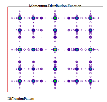
The diffraction pattern is the Fourier transform of the spatial Fibonacci array into the momentum representation.
Calculate momentum-space wave function:
\[ \Phi (p_x,~p_y) = \frac{1}{2 \pi} \sum_{m = 1}^A exp (-i p_x x_m) \sum_{n = 1}^A exp ( -i p_y y_n) \nonumber \]
Display momentum-space distribution function (diffraction pattern).
\[ \begin{matrix} \Delta = 10 & N = 200 & j = 1 .. N & px_j = - \Delta + \frac{2 \Delta j}{N} & k = 1 .. N & py_k = - \Delta + \frac{2 \Delta k}{N} \end{matrix} \nonumber \]
\[ \text{Diffraction Pattern}_{j,~k} = \left( \left| \Phi (px_j,~py_k ) \right| \right)^2 \nonumber \]
- R. Lifshitz, "The square Fibonacci tiling," Journal of Alloys and Compounds 342, 186-190 (2002).