
4.31: Calculating the Pi-electron HOMO-LUMO Electronic Transition for Benzene
- Page ID
- 151348

\( \newcommand{\vecs}[1]{\overset { \scriptstyle \rightharpoonup} {\mathbf{#1}} } \)
\( \newcommand{\vecd}[1]{\overset{-\!-\!\rightharpoonup}{\vphantom{a}\smash {#1}}} \)
\( \newcommand{\id}{\mathrm{id}}\) \( \newcommand{\Span}{\mathrm{span}}\)
( \newcommand{\kernel}{\mathrm{null}\,}\) \( \newcommand{\range}{\mathrm{range}\,}\)
\( \newcommand{\RealPart}{\mathrm{Re}}\) \( \newcommand{\ImaginaryPart}{\mathrm{Im}}\)
\( \newcommand{\Argument}{\mathrm{Arg}}\) \( \newcommand{\norm}[1]{\| #1 \|}\)
\( \newcommand{\inner}[2]{\langle #1, #2 \rangle}\)
\( \newcommand{\Span}{\mathrm{span}}\)
\( \newcommand{\id}{\mathrm{id}}\)
\( \newcommand{\Span}{\mathrm{span}}\)
\( \newcommand{\kernel}{\mathrm{null}\,}\)
\( \newcommand{\range}{\mathrm{range}\,}\)
\( \newcommand{\RealPart}{\mathrm{Re}}\)
\( \newcommand{\ImaginaryPart}{\mathrm{Im}}\)
\( \newcommand{\Argument}{\mathrm{Arg}}\)
\( \newcommand{\norm}[1]{\| #1 \|}\)
\( \newcommand{\inner}[2]{\langle #1, #2 \rangle}\)
\( \newcommand{\Span}{\mathrm{span}}\) \( \newcommand{\AA}{\unicode[.8,0]{x212B}}\)
\( \newcommand{\vectorA}[1]{\vec{#1}} % arrow\)
\( \newcommand{\vectorAt}[1]{\vec{\text{#1}}} % arrow\)
\( \newcommand{\vectorB}[1]{\overset { \scriptstyle \rightharpoonup} {\mathbf{#1}} } \)
\( \newcommand{\vectorC}[1]{\textbf{#1}} \)
\( \newcommand{\vectorD}[1]{\overrightarrow{#1}} \)
\( \newcommand{\vectorDt}[1]{\overrightarrow{\text{#1}}} \)
\( \newcommand{\vectE}[1]{\overset{-\!-\!\rightharpoonup}{\vphantom{a}\smash{\mathbf {#1}}}} \)
\( \newcommand{\vecs}[1]{\overset { \scriptstyle \rightharpoonup} {\mathbf{#1}} } \)
\( \newcommand{\vecd}[1]{\overset{-\!-\!\rightharpoonup}{\vphantom{a}\smash {#1}}} \)
\(\newcommand{\avec}{\mathbf a}\) \(\newcommand{\bvec}{\mathbf b}\) \(\newcommand{\cvec}{\mathbf c}\) \(\newcommand{\dvec}{\mathbf d}\) \(\newcommand{\dtil}{\widetilde{\mathbf d}}\) \(\newcommand{\evec}{\mathbf e}\) \(\newcommand{\fvec}{\mathbf f}\) \(\newcommand{\nvec}{\mathbf n}\) \(\newcommand{\pvec}{\mathbf p}\) \(\newcommand{\qvec}{\mathbf q}\) \(\newcommand{\svec}{\mathbf s}\) \(\newcommand{\tvec}{\mathbf t}\) \(\newcommand{\uvec}{\mathbf u}\) \(\newcommand{\vvec}{\mathbf v}\) \(\newcommand{\wvec}{\mathbf w}\) \(\newcommand{\xvec}{\mathbf x}\) \(\newcommand{\yvec}{\mathbf y}\) \(\newcommand{\zvec}{\mathbf z}\) \(\newcommand{\rvec}{\mathbf r}\) \(\newcommand{\mvec}{\mathbf m}\) \(\newcommand{\zerovec}{\mathbf 0}\) \(\newcommand{\onevec}{\mathbf 1}\) \(\newcommand{\real}{\mathbb R}\) \(\newcommand{\twovec}[2]{\left[\begin{array}{r}#1 \\ #2 \end{array}\right]}\) \(\newcommand{\ctwovec}[2]{\left[\begin{array}{c}#1 \\ #2 \end{array}\right]}\) \(\newcommand{\threevec}[3]{\left[\begin{array}{r}#1 \\ #2 \\ #3 \end{array}\right]}\) \(\newcommand{\cthreevec}[3]{\left[\begin{array}{c}#1 \\ #2 \\ #3 \end{array}\right]}\) \(\newcommand{\fourvec}[4]{\left[\begin{array}{r}#1 \\ #2 \\ #3 \\ #4 \end{array}\right]}\) \(\newcommand{\cfourvec}[4]{\left[\begin{array}{c}#1 \\ #2 \\ #3 \\ #4 \end{array}\right]}\) \(\newcommand{\fivevec}[5]{\left[\begin{array}{r}#1 \\ #2 \\ #3 \\ #4 \\ #5 \\ \end{array}\right]}\) \(\newcommand{\cfivevec}[5]{\left[\begin{array}{c}#1 \\ #2 \\ #3 \\ #4 \\ #5 \\ \end{array}\right]}\) \(\newcommand{\mattwo}[4]{\left[\begin{array}{rr}#1 \amp #2 \\ #3 \amp #4 \\ \end{array}\right]}\) \(\newcommand{\laspan}[1]{\text{Span}\{#1\}}\) \(\newcommand{\bcal}{\cal B}\) \(\newcommand{\ccal}{\cal C}\) \(\newcommand{\scal}{\cal S}\) \(\newcommand{\wcal}{\cal W}\) \(\newcommand{\ecal}{\cal E}\) \(\newcommand{\coords}[2]{\left\{#1\right\}_{#2}}\) \(\newcommand{\gray}[1]{\color{gray}{#1}}\) \(\newcommand{\lgray}[1]{\color{lightgray}{#1}}\) \(\newcommand{\rank}{\operatorname{rank}}\) \(\newcommand{\row}{\text{Row}}\) \(\newcommand{\col}{\text{Col}}\) \(\renewcommand{\row}{\text{Row}}\) \(\newcommand{\nul}{\text{Nul}}\) \(\newcommand{\var}{\text{Var}}\) \(\newcommand{\corr}{\text{corr}}\) \(\newcommand{\len}[1]{\left|#1\right|}\) \(\newcommand{\bbar}{\overline{\bvec}}\) \(\newcommand{\bhat}{\widehat{\bvec}}\) \(\newcommand{\bperp}{\bvec^\perp}\) \(\newcommand{\xhat}{\widehat{\xvec}}\) \(\newcommand{\vhat}{\widehat{\vvec}}\) \(\newcommand{\uhat}{\widehat{\uvec}}\) \(\newcommand{\what}{\widehat{\wvec}}\) \(\newcommand{\Sighat}{\widehat{\Sigma}}\) \(\newcommand{\lt}{<}\) \(\newcommand{\gt}{>}\) \(\newcommand{\amp}{&}\) \(\definecolor{fillinmathshade}{gray}{0.9}\)Calculate the wavelength of the photon required for the first allowed (HOMO-LUMO) electronic transition involving the π−electrons of benzene.
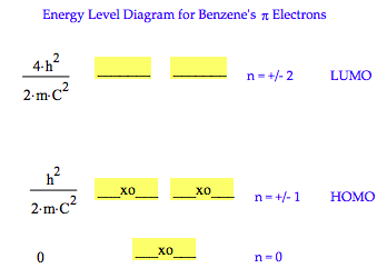
Energy conservation requirements:
\[ \frac{n_i^2 h^2}{2 m_e C^2} + \frac{hc}{ \lambda} = \frac{n_f^2 h^2}{2 m_e C^2} \nonumber \]
Fundamental constants and conversion factors:
\[ \begin{matrix} pm = 10^{-12} m & aJ = 10^{-18} J \end{matrix} \nonumber \]
\[ \begin{matrix} h = 6.6260755 (10^{-34}) \text{joule sec} & c = 2.99792458 (10^8) \frac{m}{sec} & m_e = 9.1093897 (10^{-31}) kg \end{matrix} \nonumber \]
Calculate the photon wavelength for the HOMO-LUMO electronic transition.
\[ \begin{matrix} \text{HOMO:} & n_i = 1 & \text{LUMO:} & n_f = 2 & \text{Benzene circumference:} & C = 6(140) pm \end{matrix} \nonumber \]
\[ \begin{array}{c|c} \lambda = \frac{n_i^2 h^2}{2 m_e C^2} + \frac{hc}{ \lambda} = \frac{n_f^2 h^2}{2 m_e C^2} & _{ \text{solve, } \lambda} ^{ \text{float, 3}} \rightarrow .194e-6m^3 \frac{kg}{ joule~ sec^2} ~ \lambda = 194 nm \end{array} \nonumber \]
Calculate the photon energy and frequency.
\[ \begin{matrix} \text{energy} & \frac{c}{ \lambda} = 1.024 aJ & \text{frequency} & \frac{c}{ \lambda} = 1.545 \times 10^{15} Hz \end{matrix} \nonumber \]
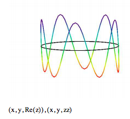
Plot Wave Functions
See Figure 7.6 (page 111) in Quantum Chemistry and Spectroscopy, by Engel.
The real part of the wave function is plotted below.
Quantum number: n = 5
\[ \begin{matrix} \text{numpts} = 100 & i = 0 .. \text{numpts} & j = 0 .. \text{numpts} & \phi_i = \frac{2 \pi i}{ \text{numpts}} \\ x_{i,~j} = \cos \left( \phi_i \right) & y_{i,~j} = \sin \left( \phi_i \right) & z_{i,~j} = \frac{1}{ \sqrt{2 \pi}} \text{exp} \left(i n \phi_i \right) & zz_{i,~j} = 0 \end{matrix} \nonumber \]
The square of the absolute magnitude for all the wave functions (for all values of the quantum number n) is 1/2π, as shown below.
\[ \begin{matrix} \left( \left| \frac{1}{ \sqrt{2 \pi}} \text{exp} (i n \phi ) \right| \right)^2 & \text{simplifies to} & \frac{1}{2 \pi} \end{matrix} \nonumber \]
The wave functions for the electron on a ring are eigenstates of the momentum operator. In other words the momentum is precisely known: p = nh/C, where n is the quantum number and C is the ring circumference. According to the uncertainty principle, the elctron position must be uncertain. The result above confirms this; the electron density is distributed uniformly over the entire ring.