3.35: Semi-empirical Molecular Orbital Calculation on XeF2

The bonding in XeF₂ can be interpreted in terms the three-center four-electron bond. In linear XeF₂ the molecular orbital can be considered to be a linear combination of the fluorine 2p orbitals and the central xenon 5p.

\[ \Psi = C_{F1} \Psi_{F1} + C_{Xe} \Psi_{Xe} + C_{F2} \Psi_{F2} \nonumber \]

Minimization of the variational integral

\[ E = \frac{ \int \left( C_{F1} \Psi_{F1} + C_{Xe} \Psi_{Xe} + C_{F2} \Psi_{F2} \right) H \left( C_{F1} \Psi_{F1} + C_{Xe} \Psi_{Xe} + C_{F2} \Psi_{F2} \right) d \tau}{ \int \left( C_{F1} \Psi_{F1} + C_{Xe} \Psi_{Xe} + C_{F2} \Psi_{F2} \right)^2 d \tau} \nonumber \]

yields the following 3 x 3 Huckel matrix

\[ H = \begin{pmatrix} \alpha_F & \beta & 0 \\ \beta & \alpha_{Xe} & \beta \\ 0 & \beta & \alpha_F \end{pmatrix} \nonumber \]

All overlap integrals are zero. The Coulomb integrals are parameterized as the negative of the valence orbital ionization energies (-12.13 eV for the Xe 5p orbital, -17.42 eV for the F 2p). The non-zero resonance integral is given a value of -2.0 eV.

\[ \begin{matrix} \alpha_{F1} = \alpha_F = \int \Psi_{F1} H \Psi_{F1} d \tau = -17.42 & \alpha_{F2} = \alpha_F = \int \Psi_{F2} H \Psi_{F2} d \tau = -17.42 \\ \alpha_{Xe} = \int \Psi_{Xe} H \Psi_{Xe} d \tau = -12.13 & \beta= \int \Psi_{Xe} H \Psi_F d \tau = -2 \end{matrix} \nonumber \]

Mathcad can now be used to find the eigenvalues and eigenvectors of H. First we must give it the values for all of the parameters.

\[ \begin{matrix} \alpha_F = -17.42 & \alpha_{Xe} = -12.13 & \beta = -2.00 \end{matrix} \nonumber \]

Define the variational matrix shown on the left side of equation (6):

\[ H = \begin{pmatrix} \alpha_F & \beta & 0 \\ \beta & \alpha_{Xe} & \beta \\ 0 & \beta & \alpha_F \end{pmatrix} \nonumber \]

Find the eigenvalues: \( \begin{matrix} \text{E = sort(eigenvals(H))} & E_0 = -18.647 & E_1 = -17.42 & E_2 = -10.903 \end{matrix}\)

Now find the eigenvectors:

\[ \begin{matrix} \text{The bonding MO is:} & \Psi_b = \text{eigenvec} \left( H,~E_0 \right) & \Psi_b = \begin{pmatrix} 0.649 \\ 0.389 \\ 0.649 \end{pmatrix} & \overrightarrow{ \left( \Psi_b \right)^2} = \begin{pmatrix} 0.421 \\ 0.158 \\ 0.421 \end{pmatrix} \\ \text{The non-bonding MO is:} & \Psi_{nb} = \text{eigenvec} \left( H,~E_1 \right) & \Psi_{nb} = \begin{pmatrix} -0.707 \\ 0 \\ 0.707 \end{pmatrix} & \overrightarrow{ \left( \Psi_{nb} \right)^2} = \begin{pmatrix} 0.5 \\ 0 \\ 0.5 \end{pmatrix} \\ \text{The anti-bonding MO is:} & \Psi_a = \text{eigenvec} \left( H,~E_2 \right) & \Psi_b = \begin{pmatrix} -0.282 \\ 0.917 \\ -0.282 \end{pmatrix} & \overrightarrow{ \left( \Psi_a \right)^2} = \begin{pmatrix} 0.079 \\ 0.842 \\ 0.079 \end{pmatrix} \end{matrix} \nonumber \]

The molecular orbital diagram for this system is shown below.

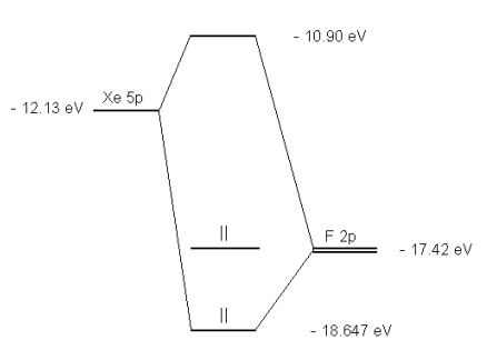
Is the molecule stable? The diagram shows two electrons each in the bonding and non-bonding orbitals for a total energy of -72.14 eV. The energy of the isolated atoms is 2(-12.13 eV) + 2(-17.42 eV) = - 59.1 eV. Thus, the molecule is more stable than the isolated atoms according to this crude semi-empirical model.

The partial charges are calculated next. The fluorine atoms have a kernel charge of +7. They get credit for 6 non-bonding atomic electrons, 42.1% of the two electrons in the bonding MO, and 50% of the two electrons in the non-bonding MO. This gives a partial charge of (7 - 6 - 2(.421) - 2(.50)) -0.842.

The xenon atom has a kernel charge of +8. It gets credit for 6 non-bonding atomic electrons, 15.8% of the two electrons in the bonding MO, and no credit for the two electrons in non-bonding MO. This yields a partial charge of (8 - 6 - 2(.158)) +1.684. This value is reasonable because xenon is bonded to the most electronegative element in the periodic table.