
3.28: A Numeric Huckel MO Calculation Using Mathcad
- Page ID
- 154423

\( \newcommand{\vecs}[1]{\overset { \scriptstyle \rightharpoonup} {\mathbf{#1}} } \)
\( \newcommand{\vecd}[1]{\overset{-\!-\!\rightharpoonup}{\vphantom{a}\smash {#1}}} \)
\( \newcommand{\dsum}{\displaystyle\sum\limits} \)
\( \newcommand{\dint}{\displaystyle\int\limits} \)
\( \newcommand{\dlim}{\displaystyle\lim\limits} \)
\( \newcommand{\id}{\mathrm{id}}\) \( \newcommand{\Span}{\mathrm{span}}\)
( \newcommand{\kernel}{\mathrm{null}\,}\) \( \newcommand{\range}{\mathrm{range}\,}\)
\( \newcommand{\RealPart}{\mathrm{Re}}\) \( \newcommand{\ImaginaryPart}{\mathrm{Im}}\)
\( \newcommand{\Argument}{\mathrm{Arg}}\) \( \newcommand{\norm}[1]{\| #1 \|}\)
\( \newcommand{\inner}[2]{\langle #1, #2 \rangle}\)
\( \newcommand{\Span}{\mathrm{span}}\)
\( \newcommand{\id}{\mathrm{id}}\)
\( \newcommand{\Span}{\mathrm{span}}\)
\( \newcommand{\kernel}{\mathrm{null}\,}\)
\( \newcommand{\range}{\mathrm{range}\,}\)
\( \newcommand{\RealPart}{\mathrm{Re}}\)
\( \newcommand{\ImaginaryPart}{\mathrm{Im}}\)
\( \newcommand{\Argument}{\mathrm{Arg}}\)
\( \newcommand{\norm}[1]{\| #1 \|}\)
\( \newcommand{\inner}[2]{\langle #1, #2 \rangle}\)
\( \newcommand{\Span}{\mathrm{span}}\) \( \newcommand{\AA}{\unicode[.8,0]{x212B}}\)
\( \newcommand{\vectorA}[1]{\vec{#1}} % arrow\)
\( \newcommand{\vectorAt}[1]{\vec{\text{#1}}} % arrow\)
\( \newcommand{\vectorB}[1]{\overset { \scriptstyle \rightharpoonup} {\mathbf{#1}} } \)
\( \newcommand{\vectorC}[1]{\textbf{#1}} \)
\( \newcommand{\vectorD}[1]{\overrightarrow{#1}} \)
\( \newcommand{\vectorDt}[1]{\overrightarrow{\text{#1}}} \)
\( \newcommand{\vectE}[1]{\overset{-\!-\!\rightharpoonup}{\vphantom{a}\smash{\mathbf {#1}}}} \)
\( \newcommand{\vecs}[1]{\overset { \scriptstyle \rightharpoonup} {\mathbf{#1}} } \)
\(\newcommand{\longvect}{\overrightarrow}\)
\( \newcommand{\vecd}[1]{\overset{-\!-\!\rightharpoonup}{\vphantom{a}\smash {#1}}} \)
\(\newcommand{\avec}{\mathbf a}\) \(\newcommand{\bvec}{\mathbf b}\) \(\newcommand{\cvec}{\mathbf c}\) \(\newcommand{\dvec}{\mathbf d}\) \(\newcommand{\dtil}{\widetilde{\mathbf d}}\) \(\newcommand{\evec}{\mathbf e}\) \(\newcommand{\fvec}{\mathbf f}\) \(\newcommand{\nvec}{\mathbf n}\) \(\newcommand{\pvec}{\mathbf p}\) \(\newcommand{\qvec}{\mathbf q}\) \(\newcommand{\svec}{\mathbf s}\) \(\newcommand{\tvec}{\mathbf t}\) \(\newcommand{\uvec}{\mathbf u}\) \(\newcommand{\vvec}{\mathbf v}\) \(\newcommand{\wvec}{\mathbf w}\) \(\newcommand{\xvec}{\mathbf x}\) \(\newcommand{\yvec}{\mathbf y}\) \(\newcommand{\zvec}{\mathbf z}\) \(\newcommand{\rvec}{\mathbf r}\) \(\newcommand{\mvec}{\mathbf m}\) \(\newcommand{\zerovec}{\mathbf 0}\) \(\newcommand{\onevec}{\mathbf 1}\) \(\newcommand{\real}{\mathbb R}\) \(\newcommand{\twovec}[2]{\left[\begin{array}{r}#1 \\ #2 \end{array}\right]}\) \(\newcommand{\ctwovec}[2]{\left[\begin{array}{c}#1 \\ #2 \end{array}\right]}\) \(\newcommand{\threevec}[3]{\left[\begin{array}{r}#1 \\ #2 \\ #3 \end{array}\right]}\) \(\newcommand{\cthreevec}[3]{\left[\begin{array}{c}#1 \\ #2 \\ #3 \end{array}\right]}\) \(\newcommand{\fourvec}[4]{\left[\begin{array}{r}#1 \\ #2 \\ #3 \\ #4 \end{array}\right]}\) \(\newcommand{\cfourvec}[4]{\left[\begin{array}{c}#1 \\ #2 \\ #3 \\ #4 \end{array}\right]}\) \(\newcommand{\fivevec}[5]{\left[\begin{array}{r}#1 \\ #2 \\ #3 \\ #4 \\ #5 \\ \end{array}\right]}\) \(\newcommand{\cfivevec}[5]{\left[\begin{array}{c}#1 \\ #2 \\ #3 \\ #4 \\ #5 \\ \end{array}\right]}\) \(\newcommand{\mattwo}[4]{\left[\begin{array}{rr}#1 \amp #2 \\ #3 \amp #4 \\ \end{array}\right]}\) \(\newcommand{\laspan}[1]{\text{Span}\{#1\}}\) \(\newcommand{\bcal}{\cal B}\) \(\newcommand{\ccal}{\cal C}\) \(\newcommand{\scal}{\cal S}\) \(\newcommand{\wcal}{\cal W}\) \(\newcommand{\ecal}{\cal E}\) \(\newcommand{\coords}[2]{\left\{#1\right\}_{#2}}\) \(\newcommand{\gray}[1]{\color{gray}{#1}}\) \(\newcommand{\lgray}[1]{\color{lightgray}{#1}}\) \(\newcommand{\rank}{\operatorname{rank}}\) \(\newcommand{\row}{\text{Row}}\) \(\newcommand{\col}{\text{Col}}\) \(\renewcommand{\row}{\text{Row}}\) \(\newcommand{\nul}{\text{Nul}}\) \(\newcommand{\var}{\text{Var}}\) \(\newcommand{\corr}{\text{corr}}\) \(\newcommand{\len}[1]{\left|#1\right|}\) \(\newcommand{\bbar}{\overline{\bvec}}\) \(\newcommand{\bhat}{\widehat{\bvec}}\) \(\newcommand{\bperp}{\bvec^\perp}\) \(\newcommand{\xhat}{\widehat{\xvec}}\) \(\newcommand{\vhat}{\widehat{\vvec}}\) \(\newcommand{\uhat}{\widehat{\uvec}}\) \(\newcommand{\what}{\widehat{\wvec}}\) \(\newcommand{\Sighat}{\widehat{\Sigma}}\) \(\newcommand{\lt}{<}\) \(\newcommand{\gt}{>}\) \(\newcommand{\amp}{&}\) \(\definecolor{fillinmathshade}{gray}{0.9}\)Enter the number of carbon atoms. \( \text{Natoms} = 4\)
Enter the number of occupied molecular orbitals. \( \text{Nocc} = 2\)
Enter the Huckel matrix.
\[ \begin{matrix} H = \begin{pmatrix} 0 & 1 & 0 & 0 \\ 1 & 0 & 1 & 0 \\ 0 & 1 & 0 & 1 \\ 0 & 0 & 1 & 0 \end{pmatrix} & H = -H \end{matrix} \nonumber \]
Calculate eigenvalues and eigenvectors:
\[ \begin{matrix} E = \text{eigenvals(H)} & \text{Display = rsort} \left( \text{stack} \left( E^T,~ \text{eigenvecs(H)} \right),~ 1 \right) \end{matrix} \nonumber \]
Display eigenvalues and eigenvectors:
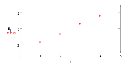
\[ \text{Display} = \begin{pmatrix} -1.618 & -0.618 & 0.618 & 1.618 \\ 0.372 & -0.602 & 0.602 & -0.372 \\ 0.602 & -0.372 & -0.372 & 0.602\\ 0.602 & 0.372 & -0.372 & -0.602 \\ 0.372 & 0.602 & 0.602 & 0.372 \end{pmatrix} \nonumber \]
Display energy level diagram. \( \begin{matrix} \text{E = sort(E)} & \text{i = 1 .. Natoms} \end{matrix}\)
Calculate total π-electronic energy:
\[ \begin{matrix} E_ \pi = 2 \sum_{i = 1} ^{ \text{Nocc}} E_i & E_ \pi = -4.472 \end{matrix} \nonumber \]
Calculate the delocalization energy:
\[ \begin{matrix} E_{deloc} = E_ \pi + 2 \text{Nocc} & E_{deloc} = -0.472 \end{matrix} \nonumber \]
Calculate the delocalization energy per atom:
\[ \frac{ \text{E}_{deloc}}{ \text{Natoms}} = -0.118 \nonumber \]
\[ C = \text{submatrix (Display, 2, Natoms + 1, 1, Natoms)} \nonumber \]
Enter the number of the molecualr orbital to be plotted.
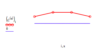
\[ \begin{matrix} r = 1 & s = 1 & 2 \sum_{i=1}^{ \text{Nocc}} \left[ \left( C^{<i>} \right)_r \left( C^{<i>} \right)_s \right] = 1 & \pi- \text{electron density on carbon 1} \\ r = 1 & s = 2 & 2 \sum_{i=1}^{ \text{Nocc}} \left[ \left( C^{<i>} \right)_r \left( C^{<i>} \right)_s \right] = 0.894 & \pi- \text{bond order between carbons 1 and 2} \\ r = 2 & s = 3 & 2 \sum_{i=1}^{ \text{Nocc}} \left[ \left( C^{<i>} \right)_r \left( C^{<i>} \right)_s \right] = 0.447 & \pi- \text{bond order between carbons 2 and 3} \\ r = 3 & s = 4 & 2 \sum_{i=1}^{ \text{Nocc}} \left[ \left( C^{<i>} \right)_r \left( C^{<i>} \right)_s \right] = 1 & \pi- \text{bond order between carbons 3 and 4} \end{matrix} \nonumber \]