3.6: The Covalent Bond According to Slater and Ruedenberg

John Slater pioneered the use of the virial theorem in interpreting the chemical bond in a benchmark paper published in the inaugural volume of the Journal of Chemical Physics (1). This early study indicated that electron kinetic energy played an important role in bond formation. Thirty years later Klaus Ruedenberg and his collaborators published a series of papers (2,3,4) detailing the crucial role that kinetic energy plays in chemical bonding, thereby completing the project that Slater started. This Mathcad worksheet recapitulates Slater's use of the virial theorem in studying chemical bond formation and summarizes Ruedenberg final analysis.

Equation [1] gives the virial theorem for a diatomic molecule as a function of internuclear separation, while equation [2] is valid at the energy minimum.

\[ 2T(R) +V(R) = =R \frac{d}{dR} E(R) \nonumber \]

\[ E \left( R_e \right) = \frac{V \left( R_e \right)}{2} = -T \left( R_e \right) \nonumber \]

At non-equilibrium values for the internuclear separation the virial equation can be used, with E = T + V, to obtain equations for the kinetic and potential energy as a function of the inter-nuclear separation.

\[ T(R) = -E(R) - R \frac{d}{dR} E(R) \nonumber \]

\[ V(R) = 2 E(R) + R \frac{d}{dR} E(R) \nonumber \]

Thus, if E(R) is known one can calculate T(R) and V(R) and provide a detailed energy profile for the formation of a chemical bond. E(R) can be provided from spectroscopic data or from ab initio quantum mechanics. In this examination of the chemical bond we employ the empirical approach and use spectroscopic data for the hydrogen molecule to obtain the parameters (highlighted below) for a model of the chemical bond based on the Morse function (5). However, it should be noted that quantum mechanics tells the same story and yields an energy profile just like that shown in the following figure.

\[ \begin{matrix} R = 30, 30.2 .. 400 & D_e = 0.761 & \beta = 0.0193 & R_e = 74.1 & E(R) = \left[ D_e \left[ 1 - \text{exp} \left[ - \beta \left( R - R_e \right) \right] \right] ^2 - D_e \right] \end{matrix} \nonumber \]

The dissociation energy, De, is given in atta (10^-18) joules, the internuclear separation in picometers, and the constant β in inverse picometers.

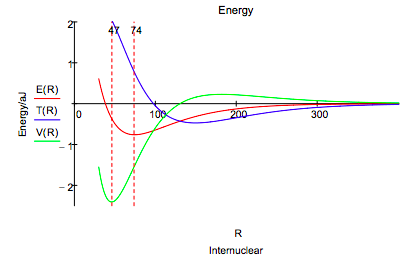
This energy profile shows that as the internuclear separation decreases, the potential energy rises, falls, and then rises again. The kinetic energy first decreases and then increases at about the same internuclear distance that the potential energy begins to decrease.

As the molecular orbital is formed at large R constructive interference between the two overlaping atomic orbitals draws electron density away from the nuclear centers into the internuclear region. The potential energy rises as electron density is drawn away from the nuclei, but the total energy decreases because of a larger decrease in kinetic energy due to charge delocalization. Thus a decrease in kinetic energy funds the initial build up of charge between the nuclei that we normally associate with chemical bond formation.

Following this initial phase, at an internuclear separation of about 180 pm the potential energy begins to decrease and the kinetic energy increases, both sharply (eventually), while the total energy continues to decrease gradually. This is an atomic effect, not a molecular one as Ruedenberg so clearly showed. The initial transfer of charge away from the nuclei and into the bond region allows the atomic orbitals to contract significantly (α increases) causing a large decrease in potential energy because the electron density has moved, on average, closer to the nuclei. The kinetic energy increases because the orbitals are smaller and kinetic energy increases inversely with the square of the orbital radius.

An energy minimum is reached while the potential energy is still in a significant decline (6), indicating that kinetic energy is the immediate cause of a stable bond and the molecular ground state in H₂. The final increase in potential energy which is due mainly to nuclear-nuclear repulsion, and not electron-electron repulsion, doesn't begin until the internuclear separation is less than 50 pm, while the equilibrium bond length is 74 pm . Thus the common explanation that an energy minimum is reached because of nuclear-nuclear repulsion does not have merit.

The H2 ground state, E = -0.761 aJ, is reached at an internuclear separation of 74 pm (1.384 a₀). In light of the previous arguments it is instructive to partition the total H₂ electron density into atomic and molecular contributions. Each electron is in a molecular orbital which is a linear combination of hydrogenic 1s orbitals, as is shown below.

\[ \begin{matrix} \Psi_{mo} = \frac{ \Psi_{1sa} + \Psi_{1sb}}{ \sqrt{2 + 2S_{ab}}} & \text{where} & \Psi_{1sa} = \sqrt{ \frac{ \alpha^3}{ \pi}} \text{exp} \left( - \alpha r_a \right) & \Psi_{1sb} = \sqrt{ \frac{ \alpha^3}{ \pi}} \text{exp} \left( - \alpha r_b \right) \end{matrix} \nonumber \]

The total electron density is therefore 2Ψ_MO². The atomic, or non-bonding, electron density is given by the following equation, which represents the electron density associated with two non-interacting atomic orbitals.

\[ \rho_n = 2 \left( \left| \frac{ \Psi_{1sa} + i \Psi_{1sb}}{ \sqrt{2}} \right| \right) = \Psi_{1sa}^2 + \Psi_{1sb}^2 \nonumber \]

Clearly, the bonding electron density must be the difference between the total electron density and the non-bonding, or atomic, electron density.

\[ \rho_b = \Psi_{MO}^2 - \rho_n = \rho_t - \rho_n \nonumber \]

These three terms are plotted along the bond axis in the figure below. Alpha is the optimum orbital scale factor, S_ab is the overlap integral, and R is the equilibrium internuclear distance in atomic units.

\[ \begin{matrix} \alpha = 1.197 & S_{ab} = 0.681 & R = 1.384 & y = 0 & z = 0 & x = -3, -2.99 .. 5 \end{matrix} \nonumber \]

\[ \rho_t ( \alpha,~x,~y,~z) = \frac{ \frac{ \alpha^2}{ \pi} \left[ \text{exp} \left( - \alpha \sqrt{x^2 + y^2+z^2} \right) + \text{exp} \left[ - \alpha \sqrt{(x-R)^2 +y^2+z^2} \right] \right]^2}{1 + S_{ab}} \nonumber \]

\[ \rho_n ( \alpha,~x,~y,~z) = \frac{ \alpha^2}{ \pi} \left[ \text{exp} \left( - \alpha \sqrt{x^2 + y^2+z^2} \right) + \text{exp} \left[ - \alpha \sqrt{(x-R)^2 +y^2+z^2} \right] \right]^2 \nonumber \]

\[ \rho_b ( \alpha,~x,~y,~z) = \rho_t ( \alpha,~x,~y,~z) - \rho_n ( \alpha,~x,~y,~z) \nonumber \]

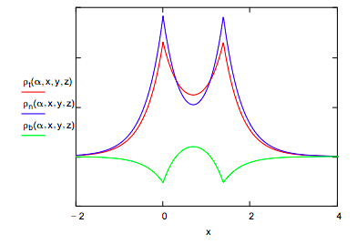
The bonding electron density illustrates that constructive interference accompanying atomic orbital overlap transfers charge from the nuclei into the internuclear region, while the non-bonding density clearly shows the subsequent atomic orbital contraction which draws some electron density back toward the nuclei.

Literature cited:

1. Slater, J. C. J. Chem. Phys. 1933, 1, 687-691.
2. Ruedenberg, K. Rev. Mod. Phys. 1962, 34, 326-352.
3. Feinberg, M. J.; Ruedenberg, K. J. Chem. Phys. 1971, 54, 1495-1511; 1971, 55, 5804-5818.
4. Feinberg, M. J.; Ruedenberg, K.; Mehler, E. L. Adv. Quantum Chem. 1970, 5, 27-98.
5. McQuarrie, D. A.; Simon, J. D. Physical Chemistry: A Molecular Approach, University Science Books, Sausalito, CA, 1997, p. 165.
6. Slater, J. C. Quantum Theory of Matter, Krieger Publishing, Huntington, N.Y., 1977, pp. 405-408.
7. Rioux, F. The Chemical Educator, 1997, 2, No. 6.