
2.45: Quantum Dots Are Artificial Atoms
- Page ID
- 158378

\( \newcommand{\vecs}[1]{\overset { \scriptstyle \rightharpoonup} {\mathbf{#1}} } \)
\( \newcommand{\vecd}[1]{\overset{-\!-\!\rightharpoonup}{\vphantom{a}\smash {#1}}} \)
\( \newcommand{\id}{\mathrm{id}}\) \( \newcommand{\Span}{\mathrm{span}}\)
( \newcommand{\kernel}{\mathrm{null}\,}\) \( \newcommand{\range}{\mathrm{range}\,}\)
\( \newcommand{\RealPart}{\mathrm{Re}}\) \( \newcommand{\ImaginaryPart}{\mathrm{Im}}\)
\( \newcommand{\Argument}{\mathrm{Arg}}\) \( \newcommand{\norm}[1]{\| #1 \|}\)
\( \newcommand{\inner}[2]{\langle #1, #2 \rangle}\)
\( \newcommand{\Span}{\mathrm{span}}\)
\( \newcommand{\id}{\mathrm{id}}\)
\( \newcommand{\Span}{\mathrm{span}}\)
\( \newcommand{\kernel}{\mathrm{null}\,}\)
\( \newcommand{\range}{\mathrm{range}\,}\)
\( \newcommand{\RealPart}{\mathrm{Re}}\)
\( \newcommand{\ImaginaryPart}{\mathrm{Im}}\)
\( \newcommand{\Argument}{\mathrm{Arg}}\)
\( \newcommand{\norm}[1]{\| #1 \|}\)
\( \newcommand{\inner}[2]{\langle #1, #2 \rangle}\)
\( \newcommand{\Span}{\mathrm{span}}\) \( \newcommand{\AA}{\unicode[.8,0]{x212B}}\)
\( \newcommand{\vectorA}[1]{\vec{#1}} % arrow\)
\( \newcommand{\vectorAt}[1]{\vec{\text{#1}}} % arrow\)
\( \newcommand{\vectorB}[1]{\overset { \scriptstyle \rightharpoonup} {\mathbf{#1}} } \)
\( \newcommand{\vectorC}[1]{\textbf{#1}} \)
\( \newcommand{\vectorD}[1]{\overrightarrow{#1}} \)
\( \newcommand{\vectorDt}[1]{\overrightarrow{\text{#1}}} \)
\( \newcommand{\vectE}[1]{\overset{-\!-\!\rightharpoonup}{\vphantom{a}\smash{\mathbf {#1}}}} \)
\( \newcommand{\vecs}[1]{\overset { \scriptstyle \rightharpoonup} {\mathbf{#1}} } \)
\( \newcommand{\vecd}[1]{\overset{-\!-\!\rightharpoonup}{\vphantom{a}\smash {#1}}} \)
\(\newcommand{\avec}{\mathbf a}\) \(\newcommand{\bvec}{\mathbf b}\) \(\newcommand{\cvec}{\mathbf c}\) \(\newcommand{\dvec}{\mathbf d}\) \(\newcommand{\dtil}{\widetilde{\mathbf d}}\) \(\newcommand{\evec}{\mathbf e}\) \(\newcommand{\fvec}{\mathbf f}\) \(\newcommand{\nvec}{\mathbf n}\) \(\newcommand{\pvec}{\mathbf p}\) \(\newcommand{\qvec}{\mathbf q}\) \(\newcommand{\svec}{\mathbf s}\) \(\newcommand{\tvec}{\mathbf t}\) \(\newcommand{\uvec}{\mathbf u}\) \(\newcommand{\vvec}{\mathbf v}\) \(\newcommand{\wvec}{\mathbf w}\) \(\newcommand{\xvec}{\mathbf x}\) \(\newcommand{\yvec}{\mathbf y}\) \(\newcommand{\zvec}{\mathbf z}\) \(\newcommand{\rvec}{\mathbf r}\) \(\newcommand{\mvec}{\mathbf m}\) \(\newcommand{\zerovec}{\mathbf 0}\) \(\newcommand{\onevec}{\mathbf 1}\) \(\newcommand{\real}{\mathbb R}\) \(\newcommand{\twovec}[2]{\left[\begin{array}{r}#1 \\ #2 \end{array}\right]}\) \(\newcommand{\ctwovec}[2]{\left[\begin{array}{c}#1 \\ #2 \end{array}\right]}\) \(\newcommand{\threevec}[3]{\left[\begin{array}{r}#1 \\ #2 \\ #3 \end{array}\right]}\) \(\newcommand{\cthreevec}[3]{\left[\begin{array}{c}#1 \\ #2 \\ #3 \end{array}\right]}\) \(\newcommand{\fourvec}[4]{\left[\begin{array}{r}#1 \\ #2 \\ #3 \\ #4 \end{array}\right]}\) \(\newcommand{\cfourvec}[4]{\left[\begin{array}{c}#1 \\ #2 \\ #3 \\ #4 \end{array}\right]}\) \(\newcommand{\fivevec}[5]{\left[\begin{array}{r}#1 \\ #2 \\ #3 \\ #4 \\ #5 \\ \end{array}\right]}\) \(\newcommand{\cfivevec}[5]{\left[\begin{array}{c}#1 \\ #2 \\ #3 \\ #4 \\ #5 \\ \end{array}\right]}\) \(\newcommand{\mattwo}[4]{\left[\begin{array}{rr}#1 \amp #2 \\ #3 \amp #4 \\ \end{array}\right]}\) \(\newcommand{\laspan}[1]{\text{Span}\{#1\}}\) \(\newcommand{\bcal}{\cal B}\) \(\newcommand{\ccal}{\cal C}\) \(\newcommand{\scal}{\cal S}\) \(\newcommand{\wcal}{\cal W}\) \(\newcommand{\ecal}{\cal E}\) \(\newcommand{\coords}[2]{\left\{#1\right\}_{#2}}\) \(\newcommand{\gray}[1]{\color{gray}{#1}}\) \(\newcommand{\lgray}[1]{\color{lightgray}{#1}}\) \(\newcommand{\rank}{\operatorname{rank}}\) \(\newcommand{\row}{\text{Row}}\) \(\newcommand{\col}{\text{Col}}\) \(\renewcommand{\row}{\text{Row}}\) \(\newcommand{\nul}{\text{Nul}}\) \(\newcommand{\var}{\text{Var}}\) \(\newcommand{\corr}{\text{corr}}\) \(\newcommand{\len}[1]{\left|#1\right|}\) \(\newcommand{\bbar}{\overline{\bvec}}\) \(\newcommand{\bhat}{\widehat{\bvec}}\) \(\newcommand{\bperp}{\bvec^\perp}\) \(\newcommand{\xhat}{\widehat{\xvec}}\) \(\newcommand{\vhat}{\widehat{\vvec}}\) \(\newcommand{\uhat}{\widehat{\uvec}}\) \(\newcommand{\what}{\widehat{\wvec}}\) \(\newcommand{\Sighat}{\widehat{\Sigma}}\) \(\newcommand{\lt}{<}\) \(\newcommand{\gt}{>}\) \(\newcommand{\amp}{&}\) \(\definecolor{fillinmathshade}{gray}{0.9}\)"A quantum dot (QD) is a nanostructure that can confine the motion of an electron in all three spatial dimensions. This gives rise to a set of discrete and narrow electronic energy levels, similar to those of atomic physics (1)."
"Essentially, artificial atoms (quantum dots) are small boxes about 100 nm on a side, contained in a semiconductor, and holding a number of electrons that may be varied at will. As in real atoms, the electrons are attracted to a central location. In a natural atom, this central location is a positively charged nucleus; in an artificial atom, electrons are typically trapped in a bowl-like parabolic potential well in which electrons tend to fall in towards the bottom of the bowl (2)."
In most cases the nanostructures resemble "pancakes" in which the electrons are restricted to motion in the x-y plane. Thus the appropriate potential is the two-dimensional harmonic oscillator.
Schrödinger's equation can be solved for this potential in both cartesian and circuluar coordinates, yielding the following expressions (in units of hν ) for the quantized energy levels. For an excellent introduction to the quantum mechanics of the two-dimensional harmonic oscillator see French & Taylor, "An Introduction to Quantum Physics," pp 454 - 463, plus three exercises on page 469.
\[ \begin{matrix} \text{E} \left( \text{n}_x,~ \text{n}_y \right) = \text{n}_x + \text{n}_y + 1 & \text{where} & \text{n}_x = 0,~1,~2,~3... & \text{and} & \text{n}_y = 0,~1,~2,~3 ... \\ \text{E} (n,~ l) = 2n+|l| + 1 & \text{where} & n = 0,~1,~3 ... & \text{and} & l = 0,~ \pm 1,~ \pm 2 ... \end{matrix} \nonumber \]
The quantum numbers and energies of the first ten states are shown in tabular format below.
\[ \begin{array}{|c|c|c|c|c|c|c|} \hline \text{n}_x & \text{n}_y & \text{E} & & n & l & \text{E} \\ \hline 0 & 0 & 1 & & 0 & 0 & 1 \\ \hline 1 & 0 & 2 & & 0 & +1 & 2 \\ \hline 0 & 1 & 2 & & 0 & -1 & 2 \\ \hline 1 & 1 & 3 & & 0 & +2 & 3 \\ \hline 2 & 0 & 3 & & 0 & -2 & 3 \\ \hline 0 & 2 & 3 & & 1 & 0 & 3 \\ \hline 3 & 0 & 4 & & 0 & +3 & 4 \\ \hline 0 & 3 & 4 & & 0 & -3 & 4 \\ \hline 1 & 2 & 4 & & 1 & +1 & 4 \\ \hline 2 & 1 & 4 & & 1 & -1 & 4 \\ \hline \end{array} \nonumber \]
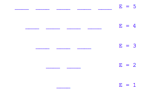
The magnitude of the energy level spacing (hν) depends on the size of the quantum dot. Each level in the diagram below can be thought of as an electronic shell and when a level is filled a new row is started in the periodic table.
According to the Pauli Exclusion principle, the first four energy levels have a capacity for 20 electrons. Assuming that there is no splitting of energy level degeneracy in multi-electron atoms, the aufbau principle would give the following structure for the periodic table for a world made up of such "pancake" atoms. The quantum numbers of the last electron added to the "atom." For example atom 4 would have four electrons and their quantum numbers would be |0 0 ½>, |0 0 - ½>, |1 0 ½>, and |0 1 ½>.
\[ \begin{matrix} 1 & & & & & & & 2 \\ | 0 ~0~ \frac{1}{2} \rangle & & & & & & & | 0 ~0 ~\frac{-1}{2} \rangle \\ 3 & 4 & &&&& 5 & 6 \\ |1~ 0 ~\frac{1}{2} \rangle & |0~ 1 ~ \frac{1}{2} \rangle & & & & & |1~0~ \frac{-1}{2} \rangle & |0 ~1~ \frac{-1}{2} \rangle \\ 7 & 8 & 9 & & & 10 & 11 & 12 \\ |1~ 1~ \frac{1}{2} \rangle & |2~ 0~ \frac{1}{2} \rangle & |0~2~ \frac{1}{2} \rangle & & & |1~ 1~ \frac{-1}{2} \rangle & |2~ 0~ \frac{-1}{2} \rangle & |0~2~ \frac{-1}{2} \rangle \\ 13 & 14 & 15 & 16 & 17 & 18 & 19 & 20 \\ |3~0~ \frac{1}{2} \rangle & |0 ~ 3~ \frac{1}{2} \rangle & |1~2~ \frac{1}{2} \rangle & |2 ~ 1~ \frac{1}{2} \rangle & |3 ~ 0 ~ \frac{-1}{2} \rangle & |0 ~ 3 ~ \frac{-1}{2} \rangle & |1 ~2 ~ \frac{-1}{2} \rangle & |2 ~ 1 ~ \frac{-1}{2} \rangle \end{matrix} \nonumber \]
To down-load a Mathcad file which will carry out a numerical integration of Schrödinger's equation click here.
To see representative wave functions click on the states shown below:
References:
- E. E. Vdovin, Science, 2000, 290, 122.
- R. C. Ashoori, Nature, 1996, 379, 413.