1.99: Visualizing the Difference Between a Superposition and a Mixture

The superposition principle, as Feynman said, is at the heart of quantum mechanics. While its mathematical expression is simple, its true meaning is difficult to grasp. For example, given a linear superposition (not normalized) of two states,

\[
|\Psi\rangle=|\phi_{1}\rangle+\left|\phi_{2}\right\rangle
\nonumber \]

one might assume that it represents a mixture of \(\phi_{1}\) and \(\phi_{2}\). In other words, half of the quons [1] are in state \(\phi_{1}\) and half in \(\phi_{2}\). However, the correct quantum mechanical interpretation of this equation is that the system represented by \(\Psi\) is simultaneously in the states \(\phi_{1}\) and \(\phi_{2}\), properly weighted.

A mixture, half \(\phi_{1}\) and half \(\phi_{2}\), or any other ratio, cannot be represented by a wavefunction. It requires a density operator, which is a more general quantum mechanical construct that can be used to represent both pure states (superpositions) and mixtures, as shown below.

\[
\hat{\rho}_{\max }=|\Psi\rangle\langle\Psi|\qquad \hat{\rho}_{\min d}=\sum p_{i}| \Psi_{i}\rangle\langle\Psi_{i}|
\nonumber \]

In the equation on the right, p_i is the fraction of the mixture in the state \(\Psi_{i}\).

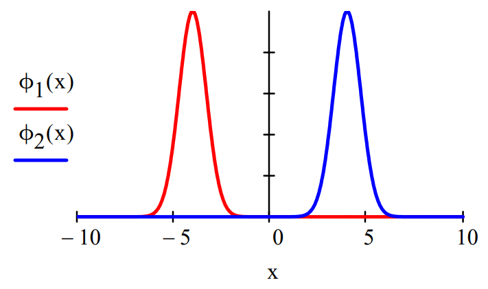
To illustrate how these equations distinguish between a mixture and a superposition, we will consider a superposition and a mixture of equally weighted gaussian functions representing one-dimensional wave packets. The normalization constants are omitted in the interest of mathematical clarity. The gaussians are centered at x = \(\pm\) 4.

\[
\phi_{1}(x) :=\exp \left[-(x+4)^{2}\right] \qquad \phi_{2}(x) :=\exp \left[-(x-4)^{2}\right]
\nonumber \]

To visualize how the density operator discriminates between a superposition and a mixture, we calculate its matrix elements in coordinate space for the 50-50 superposition and mixture of \(\phi_{1}\) and \(\phi_{2}\). The superposition is considered first.

\[
\Psi(x) :=\phi_{1}(x)+\phi_{2}(x)
\nonumber \]

The matrix elements of this pure state are calculated as follows.

\[
\rho_{\text {pure}}=\left\langle x|\hat{\rho}_{\text {pure}}| x^{\prime}\right\rangle=\langle x | \Psi\rangle\left\langle\Psi | x^{\prime}\right\rangle
\nonumber \]

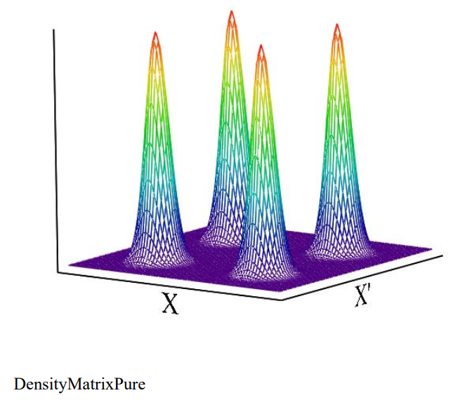
Looking at the right side we see that the matrix elements are the product of the probability amplitudes of a quon in state \(\Psi\) being at x and xʹ. Next we display the density matrix graphically.

\[
\operatorname{DensityMatrixPure}\left(x, x^{\prime}\right) :=\Psi(x) \cdot \Psi\left(x^{\prime}\right)
\nonumber \]

\[
x_{0}=8 \qquad N :=80 \qquad i :=0 \ldots N \\ \mathrm{x}_{\mathrm{i}} :=-\mathrm{x}_{0}+\frac{2 \cdot \mathrm{x}_{0} \cdot \mathrm{i}}{\mathrm{N}} \qquad \mathrm{j} :=0 \ldots \mathrm{N} \qquad \mathrm{x}_{\mathrm{j}}^{\prime} :=-\mathrm{x}_{0}+\frac{2 \cdot \mathrm{x}_{0} \cdot \mathrm{j}}{\mathrm{N}}
\nonumber \]

\[
\operatorname{DensityMatrixPure}_{\mathrm{i},\mathrm{j}} : = \operatorname{DensityMatrixPure}\left(x, x^{\prime}\right)
\nonumber \]

The presence of off-diagonal elements in this density matrix is the signature of a quantum mechanical superposition. For example, from the quantum mechanical perspective bi-location is possible.

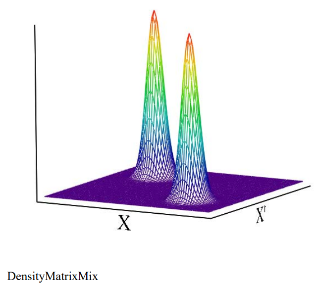
Now we turn our attention to the density matrix of a mixture of gaussian states.

\[
\rho_{\operatorname{mix}}=\left\langle x\left|\hat{\rho}_{\operatorname{mix}}\right| x^{\prime}\right\rangle=\sum_{i} p_{i}\left\langle x | \phi_{i}\right\rangle\left\langle\phi_{i} | x^{\prime}\right\rangle=\frac{1}{2}\left\langle x | \phi_{1}\right\rangle\left\langle\phi_{1} | x^{\prime}\right\rangle+\frac{1}{2}\left\langle x | \phi_{2}\right\rangle\left\langle\phi_{2} | x^{\prime}\right\rangle
\nonumber \]

\[
\operatorname{DensityMatrixMix}(\mathrm{x}, \mathrm{x'}) :=\frac{\phi_{1}(\mathrm{x}) \cdot \phi_{1}(\mathrm{x'})+\phi_{2}(\mathrm{x}) \cdot \phi_{2}\left(\mathrm{x'}^{\prime}\right)}{2}
\nonumber \]

\[
\operatorname{DensityMatrixMix}_{\mathrm{i},\mathrm{j}} : = \operatorname{DensityMatrixMix}\left(x, x^{\prime}\right)
\nonumber \]

The obvious difference between a superposition and a mixture is the absence of off-diagonal elements, \(\phi_{1}(\mathrm{x}) \cdot \phi_{2}\left(\mathrm{x}^{\prime}\right)+\phi_{2}(\mathrm{x}) \cdot \phi_{1}\left(\mathrm{x}^{\prime}\right)\), in the mixed state. This indicates the mixture is in a definite but unknown state; it is an example of classical ignorance.

An equivalent way to describe the difference between a superposition and a mixture, is to say that to calculate the probability of measurement outcomes for a superpostion you add the probability amplitudes and square the sum. For a mixture you square the individual probability amplitudes and sum the squares.

1. Nick Herbert (Quantum Reality, page 64) suggested ʺquonʺ be used to stand for a generic quantum object. ʺA quon is any entity, no matter how immense, that exhibits both wave and particle aspects in the peculiar quantum manner.