1.9: Quantum Computation- A Short Course

The Mach-Zehnder interferometer introduced above can be used to illuminate several contentious issues in quantum mechanics. The sub-microscopic building blocks of the natural world (electrons, protons, neutrons and photons) do not behave like the macroscopic objects we encounter in daily life because they have both wave and particle characteristics. Nick Herbert (Quantum Reality, p. 64) called them quons. “A quon is any entity … that exhibits both wave and particle aspects in the peculiar quantum manner.” The ‘peculiar quantum manner’ is that while we always observe particles, prior to measurement or observation quons behave like waves. This peculiar behavior is illustrated in the following tutorial.

Using a Mach-Zehnder Interferometer to Illustrate Feynman's Sum Over Histories Approach to Quantum Mechanics

Thirty-one years ago Dick Feynman told me about his 'sum over histories' version of quantum mechanics. "The electron does anything it likes," he said. "It just goes in any direction, at any speed, forward and backward in time, however it likes, and then you add up the amplitudes and it gives you the wave function." I said to him "You're crazy." But he isn't. Freeman Dyson, 1980.

In Volume 3 of the celebrated Feynman Lectures on Physics, Feynman uses the double-slit experiment as the paradigm for his 'sum over histories' approach to quantum mechanics. He said that any question in quantum mechanics could be answered by responding, "You remember the experiment with the two holes? It's the same thing." And, of course, he's right.

A 'sum over histories' is a superposition of probability amplitudes for the possible experimental outcomes which in quantum mechanics carry phase and therefore interfer constructively and destructively with one another. The square of the magnitude of the superposition of histories yields the probabilities that the various experimental possibilities will be observed.

Obviously it takes a minum of two 'histories' to demonstrate the interference inherent in the quantum mechanical superposition. And, that's why Feynman chose the double-slit experiment as the paradigm for quantum mechanical behavior. The two slits provide two paths, or 'histories' to any destination on the detection screen. In this tutorial a close cousin of the double-slit experiment, single particle interference in a Mach-Zehnder interferometer, will be used to illustrate Feynman's 'sum over histories' approach to quantum mechanics.

A Beam Splitter Creates a Quantum Mechanical Superposition

Single photons emitted by a source (S) illuminate a 50-50 beam splitter (BS). Mirrors (M) direct the photons to detectors D₁ and D₂. The probability amplitudes for transmission and reflection are given below. By convention a 90 degree phase shift (i) is assigned to reflection.

Probability amplitude for photon transmission at a 50-50 beam splitter:

\[
\langle T | S\rangle=\frac{1}{\sqrt{2}}
\nonumber \]

Probability amplitude for photon reflection at a 50-50 beam splitter:

\[
\langle R | S\rangle=\frac{i}{\sqrt{2}}
\nonumber \]

After the beam splitter the photon is in a superposition state of being transmitted and reflected.

\[
| S \rangle \rightarrow \frac{1}{\sqrt{2}} \left[ |T\rangle+ i | R \rangle \right]
\nonumber \]

As shown in the diagram below, mirrors reflect the transmitted photon path to D₂ and the reflected path to D₁. The source photon is expressed in the basis of the detectors as follows.

\[
| S \rangle \rightarrow \frac{1}{\sqrt{2}}[ |T\rangle+ i | R \rangle ] \xrightarrow[R \rightarrow D_{1}]{T \rightarrow D_{2}}>\frac{1}{\sqrt{2}}[ |D_{2}\rangle+ i | D_{1} \rangle ]
\nonumber \]

The square of the magnitude of the coefficients of D₁ and D₂ give the probabilities that the photon will be detected at D₁ or D₂. Each detector registers photons 50% of the time. In other words, in the quantum view the superposition collapses randomly to one of the two possible measurement outcomes it represents.

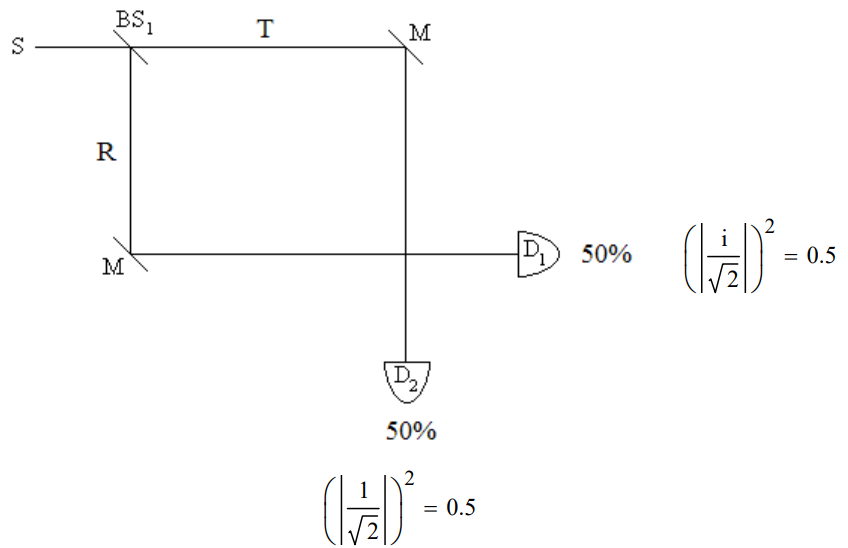
The classical view that detection at D₁ means the photon was reflected at BS₁ and that detection at D₂ means it was transmitted at BS₁ is not tenable as will be shown using a Mach-Zehnder interferometer which has a second beam splitter at the path intersection before the detectors.

A Second Beam Splitter Provides Two Paths to Each Detector

If a second beam splitter is inserted before the detectors the photons always arrive at D₁. In the first experiment there was only one path to each detector. The construction of a Mach-Zehnder interferometer by the insertion of a second beam splitter creates a second path to each detector and the opportunity for constructive and destructive interference on the paths to the detectors.

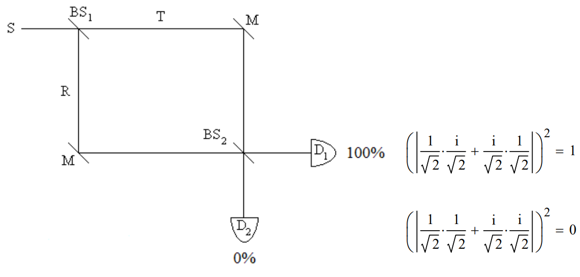
Given the superposition state after BS₁, the probability amplitudes after BS₂ interfere constructively at D₁ and destructively at D₂.

\[\begin{matrix} \text{After BS}_{1} & \text{After BS}_{2} & \text{Final State} \\ \; & | T \rangle \rightarrow \frac{1}{\sqrt{2}}[i | D_{1}\rangle+| D_{2} \rangle ] & \; \\ | S \rangle \rightarrow \frac{1}{\sqrt{2}}[ |T\rangle+ i | R \rangle ] \rightarrow & + & \rightarrow \quad i | D_{1} \rangle \\ \; & i | R \rangle \rightarrow \frac{i}{\sqrt{2}}[ |D_{1}\rangle+ i | D_{2} \rangle ] & \; \end{matrix} \nonumber \]

Adopting the classical view that the photon is either transmitted or reflected at BS₁ does not produce this result. If the photon was transmitted at BS₁ it would have equal probability of arriving at either detector after BS₂. If the photon was reflected at BS₁ it would also have equal probability of arriving at either detector after BS₂. The predicted experimental results would be the same as those of the single beam splitter experiment. In summary, the quantum view that the photon is in a superposition of being transmitted and reflected after BS₁ is consistent with both experimental results described above; the classical view that it is either transmitted or reflected is not.

Some disagree with this analysis saying the two experiments demonstrate the dual, complementary, behavior of photons. In the first experiment particle-like behavior is observed because both detectors register photons indicating the individual photons took one path or the other. The second experiment reveals wave-like behavior because interference occurs - only D₁ registers photons. According to this view the experimental design determines whether wave or particle behavior will occur and somehow the photon is aware of how it should behave. Suppose in the second experiment that immediately after the photon has interacted with BS₁, BS₂ is removed. Does what happens at the detectors require the phenomenon of retrocausality or delayed choice? Only if you reason classically about quantum experiments.

We always measure particles (detectors click, photographic film is darkened, etc.) but we interpret what happened or predict what will happen by assuming wavelike behavior, in this case the superposition created by the initial beam splitter that delocalizes the position of the photon. Quantum particles (quons) exhibit both wave and particle properties in every experiment. To paraphrase Nick Herbert (Quantum Reality), particles are always detected, but the experimental results observed are the result of wavelike behavior. Richard Feynman put it this way (The Character of Physical Law), "I will summarize, then, by saying that electrons arrive in lumps, like particles, but the probability of arrival of these lumps is determined as the intensity of waves would be. It is in this sense that the electron behaves sometimes like a particle and sometimes like a wave. It behaves in two different ways at the same time (in the same experiment)." Bragg said, "Everything in the future is a wave, everything in the past is a particle."

In 1951 in his treatise Quantum Theory, David Bohm described wave-particle duality as follows: "One of the most characteristic features of the quantum theory is the wave-particle duality, i.e. the ability of matter or light quanta to demonstrate the wave-like property of interference, and yet to appear subsequently in the form of localizable particles, even after such interference has taken place." In other words, to explain interference phenomena wave properties must be assigned to matter and light quanta prior to detection as particles.

Matrix Mechanics Approach

As a companion analysis, the matrix mechanics approach to single-photon interference in a Mach-Zehnder interferometer is outlined next.

State Vectors

Photon moving horizontally:

\[
\mathrm{x} :=\left( \begin{array}{l}{1} \\ {0}\end{array}\right)
\nonumber \]

Photon moving vertically:

\[
\mathrm{y} :=\left( \begin{array}{l}{0} \\ {1}\end{array}\right)
\nonumber \]

Operators

Operator representing a beam splitter:

\[
\mathrm{BS} :=\frac{1}{\sqrt{2}} \cdot \left( \begin{array}{cc}{1} & {\mathrm{i}} \\ {\mathrm{i}} & {1}\end{array}\right)
\nonumber \]

Operator representing a mirror:

\[
\mathrm{M} :=\left( \begin{array}{ll}{0} & {1} \\ {1} & {0}\end{array}\right)
\nonumber \]

Single beam splitter example:

Reading from right to left.

The probability that a photon leaving the source moving in the (horizontal) x-direction, encountering a beam splitter and a mirror will be detected at D1.	$$ \left(\left|x^{\mathrm{T}} \cdot \mathrm{M} \cdot \mathrm{BS} \cdot \mathrm{x}\right|\right)^{2}=0.5 $$
The probability that a photon leaving the source moving in the (horizontal) x-direction, encountering a beam splitter and a mirror will be detected at D2.	$$ \left(\left|y^{\mathrm{T}} \cdot \mathrm{M} \cdot \mathrm{BS} \cdot \mathrm{x}\right|\right)^{2}=0.5 $$

Two beam splitter example (MZI):

The probability that a photon leaving the source moving in the (horizontal) x-direction, encountering a beam splitter, a mirror and another beam splitter will be detected at D1.	$$ \left(\left|\mathrm{x}^{\mathrm{T}} \cdot \mathrm{BS} \cdot \mathrm{M} \cdot \mathrm{BS} \cdot \mathrm{x}\right|\right)^{2}=1 $$
The probability that a photon leaving the source moving in the (horizontal) x-direction, encountering a beam splitter, a mirror and another beam splitter will be detected at D2.	$$ \left(\left|y^{\mathrm{T}} \cdot \mathrm{BS} \cdot \mathrm{M} \cdot \mathrm{BS} \cdot \mathrm{x}\right|\right)^{2}=0 $$

Some quantum physicists believe they can isolate wave and particle behavior in a properly designed experiment. They also invoke the concept of delayed choice. I disagree with both in the next tutorial, but first some remarks by John Wheeler.

John Wheeler, designer of several delayed-choice experiments (both terrestrial and cosmological), had the following to say about the interpretation of such experiments.

... in a loose way of speaking, we decide what the photon shall have done after it has already done it. In actuality it is wrong to talk of the ʹrouteʹ of the photon. For a proper way of speaking we recall once more that it makes no sense to talk of a phenomenon until it has been brought to a close by an irreversible act of amplification. ‘No elementary phenomenon is a phenomenon until it is a registered (observed) phenomenon.’

A Quantum Delayed-Choice Experiment?

This note presents a critique of "Entanglement-Enabled Delayed-Choice Experiment," F. Kaiser, et al. Science 338, 637 (2012). This experiment was also summarized in section 6.3 of Quantum Weirdness, by William Mullin, Oxford University Press, 2017.

A source, S, emits two photons in opposite directions on the x-axis in the following polarization state, where v and h represent vertical and horizontal polarization, respectively.

\[
| \Psi \rangle_{A B}=\frac{1}{\sqrt{2}}[ |x \nu \rangle_{A} | x \nu \rangle_{B}+| x h \rangle_{A} | x h \rangle_{B} ]
\nonumber \]

Photon B travels to the left to a polarizing beam splitter, PBS. Photon A travels to the right entering an interferometer whose elements are a beam splitter (BS), two mirrors (M), and a polarization-dependent beam splitter (PDBS).

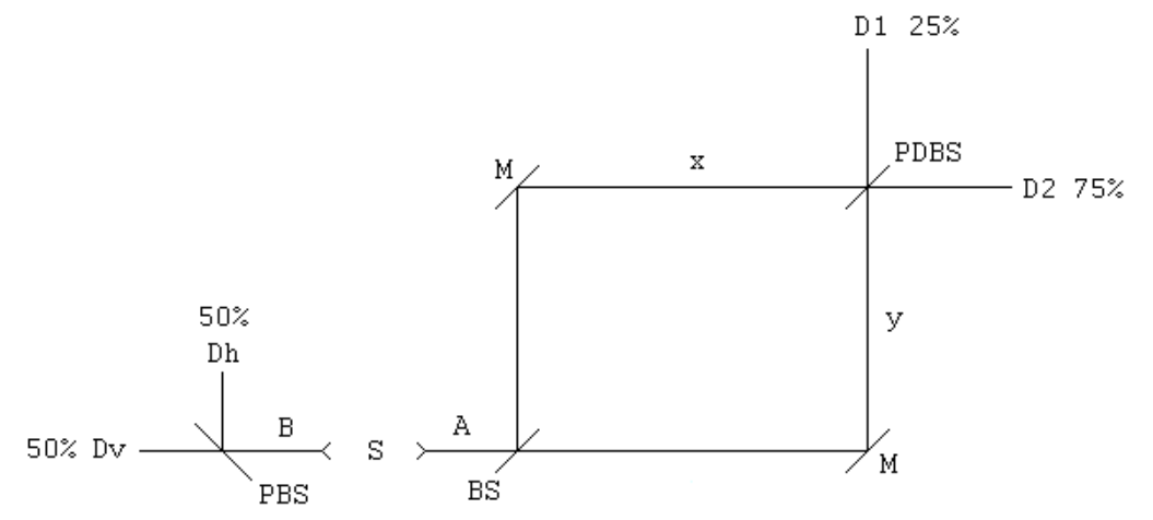
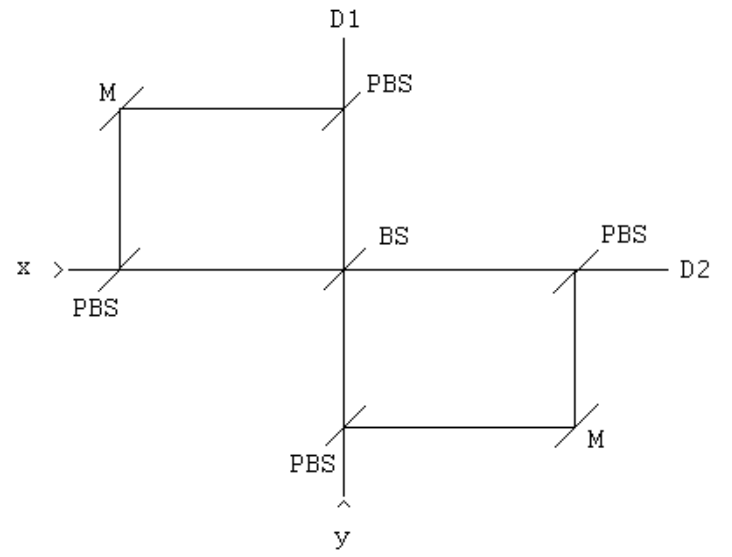
The implementation of the PDBS is shown here.

The operation of the optical elements are as follows. A mirror simply reflects the photon's direction of motion.

\[
M=| y \rangle\langle x|+| x\rangle\langle y|
\nonumber \]

A 50-50 BS splits the photon beam into a superposition of motion in the x- and y-directions. By convention the reflected beam collects a pi/2 (i) phase shift relative to the transmitted beam.

\[
B S=\frac{ |x \rangle+i | y\rangle}{\sqrt{2}}\langle x|+\frac{i | x \rangle+| y\rangle}{\sqrt{2}}\langle y|=\frac{1}{\sqrt{2}}( |x\rangle\langle x|+i| y\rangle\langle x|+i| x\rangle\langle y|+| y\rangle\langle y|)
\nonumber \]

A PBS transmits vertically polarized photons and reflects horizontally polarized photons.

\[
P B S=| x v \rangle\langle x v|+| y h\rangle\langle x h|+| y v\rangle\langle y v|+| x h\rangle\langle y h|
\nonumber \]

The PDBS uses an initial PBS to reflect horizontally polarized photons to a second PBS which reflects them to the detectors. Vertically polarized photons are transmitted by the first PBS to a BS which has the action shown above, after which they are transmitted to the detectors by the second PBS. PBS/PDBS blue/red color coding highlights the action of the central BS.

\[
P D P S=\frac{ |x v \rangle+i | y v\rangle}{\sqrt{2}}\langle x v|+| y h\rangle\langle x h|+\frac{i | x v \rangle+| y v\rangle}{\sqrt{2}}\langle y v|+| x h\rangle\langle y h|
\nonumber \]

Given the state produced by the source, half the time a horizontal photon will enter the interferometer and half the time a vertical photon will enter. The following algebraic analysis shows the progress of the h- and v-polarized photons entering the interferometer. It is clear from this analysis that D1 will fire 25% of the time and D2 75% of the time.

\[\begin{matrix} | xh \rangle & | x \nu \rangle \\ BS & BS \\ \frac{ |x h \rangle+i | y h\rangle}{\sqrt{2}} & \frac{ |x v \rangle+i | y v\rangle}{\sqrt{2}} \\ M & M \\ \frac{ |y h \rangle+i | x h\rangle}{\sqrt{2}} & \frac{ |y v \rangle+i | x v\rangle}{\sqrt{2}} \\ PDBS & PDBS \\ \frac{ |D 2 \rangle | h \rangle+i | D 1 \rangle | h\rangle}{\sqrt{2}} & \frac{1}{\sqrt{2}}\left[\frac{ |D 1 \rangle | v \rangle+i | D 2 \rangle | v\rangle}{\sqrt{2}}+\frac{i(i | D 1\rangle | v \rangle+| D 2 \rangle | v\rangle )}{\sqrt{2}}\right] \\ \; & \downarrow \\ \; & i | D 2 \rangle | v \rangle \end{matrix} \nonumber \]

This analysis suggests to some that inside the interferometer h-photons behave like particles and v-photons behave like waves. The argument for this view is that interference occurs at the PDBS for v-photons, but not for h-photons. However, in both cases the state illuminating the PDBS, highlighted in blue, is a superposition of the photon being in both arms of the interferometer. In my opinion this superposition implies delocalization which implies wavelike behavior. At the PDBS the h-photon superposition is reflected away from the central BS to D1 and D2, leading to the final superposition in the left-hand column above, which collapses on observation to either D1 or D2. The v-photon superposition is transmitted at the PDBS to the central BS allowing for destructive interference at D1 and constructive interference at D2 as is shown at the bottom of the right-hand column.

Those who interpret this experiment in terms of particle or wave behavior also invoke the concept of delayed-choice, claiming that if D2 fires we don't know for sure which behavior has occurred because both h and v photons can arrive there. They argue that until photon B has been observed at Dv or Dh, which by design can be long after photon A has exited the interferometer, the polarization of the photon detected at D2 is unknown and therefore so is whether particle or wave behavior has occurred. These analysts write the final two photon wavefunction as the following entangled superposition, where particle behavior is highlighted in red and wave behavior in blue.

\[
\begin{split}| \Psi \rangle_{\text {final}}&=\frac{1}{\sqrt{2}} \left(\left(\frac{ |D 2, h \rangle+i | D 1, h\rangle}{\sqrt{2}}\right)_{A} | D h\rangle_{B}+i | D 2, \nu \rangle_{A} | D \nu \rangle_{B}\right )\\&=\frac{1}{\sqrt{2}}( |Particle\rangle_{A} | D h \rangle_{B}+| W a v e \rangle_{A} | D v \rangle_{B} ) \end{split}
\nonumber \]

For the reasons expressed above I do not find this interpretation convincing. We always observe particles (detectors click, photographic film is darkened, etc.), but we interpret what happened or predict what will happen by assuming wavelike behavior. In other words, objects governed by quantum mechanical principles (quons) exhibit both wave and particle properties in every experiment. To paraphrase Nick Herbert (Quantum Reality), particles are always detected, but the experimental results observed are the result of wavelike behavior. Bragg summarized wave-particle duality saying, "Everything in the future is a wave, everything in the past is a particle."

In summary, I accept the Copenhagen interpretation of quantum mechanics for the reasons so cogently stated by David Lindley on page 164 of Where Does The Weirdness Go?

And since none of the other “interpretations” of quantum mechanics that we have looked at has brought us any real peace of mind, they simply push the weirdness around, from one place to another, but cannot make it go away – let us stick with the Copenhagen interpretation, which has the virtues of simplicity and necessity. It takes quantum mechanics seriously, takes its weird aspects at face value, and provides an economical, austere, perhaps even antiseptic, account of them.

We now turn to some true quantum weirdness. The following tutorial uses a Mach-Zehnder interferometer (MZI) and Feynman’s sum over histories approach to demonstrate interaction-free measurement, or how to see in the dark.

Interaction Free Measurement: Seeing in the Dark

The illustration of the concept of interaction-free measurement requires the use of an interferometer. A simple illustration employs a Mach-Zehnder interferometer (MZI) like the one shown here.

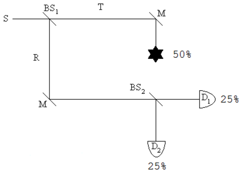
This equal-arm MZI consists of two 50-50 beam splitters (BS₁, BS₂), two mirrors (M) and two detectors (D₁, D₂). A source emits a photon which interacts with BS₁ producing the following superposition. (By convention a 90 degree (i) phase shift is assigned to reflection.)

\[
\mathrm{S}=\frac{1}{\sqrt{2}} \cdot(\mathrm{T}+\mathrm{i} \cdot \mathrm{R}) \tag{1}
\nonumber \]

The transmitted and reflected branches are united at BS₂ by the mirrors, where they evolve into the following superpositions in the basis of the detectors.

\[
\mathrm{T}=\frac{1}{\sqrt{2}} \cdot\left(\mathrm{i} \cdot \mathrm{D}_{1}+\mathrm{D}_{2}\right) \tag{2}
\nonumber \]

\[
\mathrm{R}=\frac{1}{\sqrt{2}} \cdot\left(\mathrm{D}_{1}+\mathrm{i} \cdot \mathrm{D}_{2}\right) \tag{3}
\nonumber \]

Substitution of 2 and 3 into 1 reveals that the output photon is always registered at D₁. There are two paths to each detector and constructive interference occurs at D₁ and destructive interference at D₂.

\[
\mathrm{S}=\frac{1}{\sqrt{2}} \cdot(\mathrm{T}+\mathrm{i} \cdot \mathrm{R}) \Bigg|^{\text { substitute, } \mathrm{T}=\frac{1}{\sqrt{2}} \cdot\left(\mathrm{i} \cdot \mathrm{D}_{1}+\mathrm{D}_{2}\right)}_{\text { substitute, } \mathrm{R}=\frac{1}{\sqrt{2}} \cdot\left(\mathrm{D}_{1}+\mathrm{i} \cdot \mathrm{D}_{2}\right)}\rightarrow \mathrm{S}=\mathrm{D}_{1} \cdot \mathrm{i}
\nonumber \]

Probability at D₁:

\[
(|i|)^{2}=1
\nonumber \]

The MZI provides a rudimentary method of determining whether an obstruction is present in its upper arm without actually interacting with it. As we shall see, it is not an efficient method, but it does clearly illustrate the principle involved which then can be used in a more elaborate and sophisticated interferometer to yield better results.

In the presence of the obstruction equation 2 becomes \(T = \gamma_{Absorbed}\). This leads to the following result at the detectors.

\[
\mathrm{s}=\frac{1}{\sqrt{2}} \cdot(\mathrm{T}+\mathrm{i} \cdot \mathrm{R}) \Bigg|^{\text { substitute, } \mathrm{T}=\gamma_{\mathrm{Absorbed}}}_{\text { substitute, } \mathrm{R}=\frac{1}{\sqrt{2}} \cdot\left(\mathrm{D}_{1}+\mathrm{i} \cdot \mathrm{D}_{2}\right)} \rightarrow \mathrm{S}=\frac{\sqrt{2} \cdot \gamma_{\mathrm{Absorbed}}}{2}-\frac{\mathrm{D}_{2}}{2}+\frac{\mathrm{D}_{1} \mathrm{i}}{2}
\nonumber \]

Quantum mechanics predicts that for a large number of experiments 50% of the photons will be absorbed by the obstruction, 25% will be detected at D₁ and 25% will be detect at D₂. This later result is the signature of interaction-free measurement. Even if the photon is not absorbed, the mere presence of the obstruction causes the probability of detection at D₂ to go from zero to 25%. The photon's arrival at D₂ signals the presence of an obstruction in the upper arm of the MZI, and the obstruction is detected without an interaction.

Of course, 25% is not great efficiency, so this is "a proof of principle" example. However, with a little ingenuity the probability of interaction-free detection can be increased dramatically. To see how this can be accomplished read "Quantum Seeing in the Dark" by Kwiat, Weinfurter and Zeilinger in the November 1996 issue of Scientific American.

However, it is possible to improve performance significantly by using a system of nested MZIs which is only slightly more complicated than the simple MZI used earlier. To simplify analysis Feynman's "sum over histories" approach to quantum mechanics will be used. The probability amplitudes for transmission and reflection at the beam splitters are required.

\[
\mathrm{T} :=\frac{1}{\sqrt{2}} \qquad \mathrm{R} :=\frac{\mathrm{i}}{\sqrt{2}}
\nonumber \]

Placing an additional BS before the original MZI and another BS before D₂ and renaming it D₃, plus an additional mirror and new detector D₂, yields a nested interferometer configuration that significantly increases the probability of interaction-free detection of the obstruction.

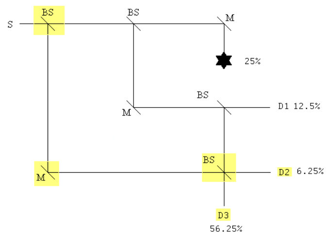
To interact with the obstruction a photon must be transmitted at the first and second beam splitters. In this case there is only one history and the probability of the interaction occuring is the square of its absolute magnitude.

\[
(|\mathrm{T} \cdot \mathrm{T}|)^{2} \rightarrow \frac{1}{4}=25 \%
\nonumber \]

The probabilities of detectors 1, 2 and 3 firing are calculated using the same methodology.

The probability D₁ registers a photon:

\[
(|\mathrm{T} \cdot \mathrm{R} \cdot \mathrm{T}|)^{2} \rightarrow \frac{1}{8}=12.5 \%
\nonumber \]

The probability D₂ registers a photon:

\[
(|\mathrm{T} \cdot \mathrm{R} \cdot \mathrm{R} \cdot \mathrm{R}+\mathrm{R} \cdot \mathrm{T}|)^{2} \rightarrow \frac{1}{16}=6.25 \%
\nonumber \]

The probability D₃ registers a photon:

\[
(|\mathrm{T} \cdot \mathrm{R} \cdot \mathrm{R} \cdot \mathrm{T}+\mathrm{R} \cdot \mathrm{R}|)^{2} \rightarrow \frac{9}{16}=56.25 \%
\nonumber \]

With the modified interferometer detecting the presence of the obstruction without interacting with it increases from 25% to 56.25%.

Perhaps weirder is the quantum Cheshire cat. The following tutorial shows how a MZI can be engineered to create a situation in which a photon is separated from a property, in this case its angular momentum.

A Quantum Optical Cheshire Cat

The following is a summary of "Quantum Cheshire Cats" by Aharonov, Popescu, Rohrlich and Skrzypczyk which was published in the New Journal of Physics 15, 113015 (2013) and can also be accessed at: arXiv:1202.0631v2.

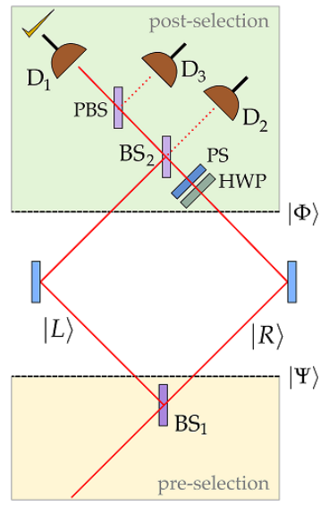
In the absence of the half-wave plate (HWP) and the phase shifter (PS) a horizontally polarized photon entering the interferometer from the lower left (propagating to the upper right) arrives at D₂ with a 90 degree (\(\frac{\pi}{2}, i\)) phase shift. (By convention reflection at a beam splitter introduces a 90 degree phase shift.)

\[
| R \rangle | H \rangle \stackrel{B S_{i}}{\longrightarrow} \frac{1}{\sqrt{2}}[i | L\rangle+| R \rangle ] | H \rangle \stackrel{B s_{2}}{\longrightarrow} i | D_{2} \rangle | H \rangle
\nonumber \]

The state immediately after the first beam splitter is the pre-selected state.

\[
| \Psi \rangle=\frac{1}{\sqrt{2}}[i | L\rangle+| R \rangle ] | H \rangle
\nonumber \]

The post-selected state is,

\[
| \Phi \rangle=\frac{1}{\sqrt{2}}[ |L\rangle | H \rangle+| R \rangle | V \rangle ]
\nonumber \]

The HWP (converts |V> to |H> in the R-branch) and PS transform this state to,

\[
| \Phi \rangle \xrightarrow[P S]{H W P}\frac{1}{\sqrt{2}}[ |L\rangle+ i | R \rangle ] | H \rangle
\nonumber \]

which exits the second beam splitter through the left port to encounter a polarizing beam splitter which transmits horizontal polarization and reflects vertical polarization. Thus, the post-selected state is detected at D₁. The evolution of the post-selected state is summarized as follows:

\[
| \Phi \rangle=\frac{1}{\sqrt{2}}[ |L\rangle | H \rangle+| R \rangle | V \rangle ] \xrightarrow[P S]{H W P}[ |L\rangle+ i | R \rangle ] | H \rangle \xrightarrow{B S_{2}} i | L \rangle | H \rangle \xrightarrow{P B S} i | D_{1} \rangle | H \rangle
\nonumber \]

The last term on the right side below is the weak value of A multiplied by the probability of its occurrence for the preselected state \(\Psi\) and the post-selected state \(\Phi\).

\[
\langle\Psi|\widehat{\mathrm{A}}| \Psi\rangle=\sum_{j}\langle\Psi | \Phi_{j}\rangle\left\langle\Phi_{j}|\hat{\mathrm{A}}| \Psi\right\rangle=\sum_{j}\langle\Psi | \Phi_{j}\rangle\left\langle\Phi_{j} | \Psi\right\rangle \frac{\left\langle\Phi_{j}|\hat{\mathbf{A}}| \Psi\right\rangle}{\left\langle\Phi_{j} | \Psi\right\rangle}=\sum_{j} p_{j} \frac{\left\langle\Phi_{j}|\hat{\mathbf{A}}| \Psi\right\rangle}{\left\langle\Phi_{j} | \Psi\right\rangle}
\nonumber \]

The weak value calculations are carried out in a 4-dimensional Hilbert space created by the tensor product of the photon's direction of propagation and polarization vectors.

Direction of propagation vectors:

\[
\mathrm{L} :=\left( \begin{array}{l}{1} \\ {0}\end{array}\right) \qquad \mathrm{R} :=\left( \begin{array}{l}{0} \\ {1}\end{array}\right)
\nonumber \]

Polarization state vectors:

\[
\mathrm{H} :=\left( \begin{array}{l}{1} \\ {0}\end{array}\right) \qquad \mathrm{V} :=\left( \begin{array}{l}{0} \\ {1}\end{array}\right)
\nonumber \]

Pre-selected state:

\[
\Psi=\frac{1}{\sqrt{2}} \cdot(i \cdot L+R) \cdot H=\frac{1}{\sqrt{2}} \cdot\left[i \cdot \left( \begin{array}{l}{1} \\ {0}\end{array}\right)+\left( \begin{array}{l}{0} \\ {1}\end{array}\right)\right] \cdot \left( \begin{array}{l}{1} \\ {0}\end{array}\right)=\frac{1}{\sqrt{2}} \cdot \left( \begin{array}{l}{i} \\ {1}\end{array}\right) \cdot \left( \begin{array}{l}{i} \\ {0}\end{array}\right) \qquad \Psi :=\frac{1}{\sqrt{2}} \cdot \left( \begin{array}{l}{i} \\ {0} \\ {1} \\ {0}\end{array}\right)
\nonumber \]

Post-selected state:

\[
\Phi :=\frac{1}{\sqrt{2}} \cdot(\mathrm{L} \cdot \mathrm{H}+\mathrm{R} \cdot \mathrm{V})=\frac{1}{\sqrt{2}} \cdot\left[\left( \begin{array}{l}{1} \\ {0}\end{array}\right) \cdot \left( \begin{array}{l}{1} \\ {0}\end{array}\right)+\left( \begin{array}{l}{0} \\ {1}\end{array}\right) \cdot \left( \begin{array}{l}{0} \\ {1}\end{array}\right)\right] \qquad \Phi :=\frac{1}{\sqrt{2}} \cdot \left( \begin{array}{l}{1} \\ {0} \\ {0} \\ {1}\end{array}\right)
\nonumber \]

Direction of propagation operators:

\[
\text{Left}:=\left( \begin{array}{l}{1} \\ {0}\end{array}\right) \cdot \left( \begin{array}{ll}{1} & {0}\end{array}\right) \rightarrow \left( \begin{array}{ll}{1} & {0} \\ {0} & {0}\end{array}\right) \qquad \text{Right}:=\left( \begin{array}{l}{0} \\ {1}\end{array}\right) \cdot \left( \begin{array}{cc}{0} & {1}\end{array}\right) \rightarrow \left( \begin{array}{ll}{0} & {0} \\ {0} & {1}\end{array}\right)
\nonumber \]

Photon angular momentum operator:

\[
\operatorname{Pang} :=\left( \begin{array}{cc}{0} & {-i} \\ {i} & {0}\end{array}\right)
\nonumber \]

Identity operator:

\[
\mathrm{I} :=\left( \begin{array}{ll}{1} & {0} \\ {0} & {1}\end{array}\right)
\nonumber \]

The following weak value calculations show that for the pre- and post-selection ensemble of observations the photon is in the left arm of the interferometer while its angular momentum is in the right arm. Like the case of the Cheshire cat, a photon property has been separated from the photon.

\[\begin{pmatrix} \; & \text{“Left Arm''} & \text{“Right Arm''} \\ \text{ “Arm''} & \frac{\Phi^{\mathrm{T}} \cdot \text { kronecker }(\mathrm{Left}, 1) \cdot \Psi}{\Phi^{\mathrm{T}} \cdot \Psi} & \frac{\Phi^{\mathrm{T}} \cdot \text { kronecker }(\mathrm{Right}, \mathrm{I}) \cdot \Psi}{\mathbf{\Phi}^{\mathrm{T}} \cdot \Psi} \\ \text{ “Pang''} & \frac{\Phi^{\mathrm{T}} \cdot \text { kronecker (Left, Pang) } \cdot \Psi}{\Phi^{\mathrm{T}} \cdot \Psi} & \frac{\Phi^{\mathrm{T}} \cdot \text { kronecker (Right }, \text { Pang } ) \cdot \Psi}{\Phi^{\mathrm{T}} \cdot \Psi} \end{pmatrix}= \begin{pmatrix} \; & \text{ “Left Arm''} & \text{ “Right Arm''} \\ \text{ “Arm''} & 1 & 0 \\ \text{ “Pang''} & 0 & 1 \end{pmatrix} \nonumber \]

The following shows the evolution of the pre-selected state to the final state at the detectors. The intermediate is the state illuminating BS₂. The polarization state at the detectors is ignored.

\[
| \Psi \rangle \rightarrow \frac{i}{\sqrt{2}}[ |L\rangle | H \rangle+| R \rangle | V \rangle ] \rightarrow-\frac{1}{2} | D_{1} \rangle+\frac{i}{2} | D_{3} \rangle+\frac{(i-1)}{2} | D_{2} \rangle
\nonumber \]

Squaring the magnitude of the probability amplitudes shows that the probabilities that D₁, D₃ and D₂ will fire are 1/4, 1/4 and 1/2, respectively. The probability at D₁ is consistent with the probability that the post-selected state is contained in the pre-selected state. A photon in the post-selected state has a probability of 1 of reaching D₁ and it represents a 25% contribution to the pre-selected state.

\[
\left(\left|\Phi^{\mathrm{T}} \cdot \Psi\right|\right)^{2} \rightarrow \frac{1}{4}
\nonumber \]

Note that the expectation values for the pre-selected state show no path-polarization separation.

\[\left[ \begin{matrix} \; & \text{ “Left Arm''} & \text{ “Right Arm''} \\ \text{ “Arm''} & \left(\overline{\Psi}\right)^{\mathrm{T}} \cdot \text { kronecker (Left, } \mathrm{I} ) \cdot \Psi & \left(\overline{\Psi}\right)^{\mathrm{T}} \cdot \text { kronecker (Right, } \mathrm{I} ) \cdot \Psi \\ \text{ “Pang''} & \left(\overline{\Psi}\right)^{\mathrm{T}} \cdot \text { kronecker (Left, } \mathrm{Pang} ) \cdot \Psi & \left(\overline{\Psi}\right)^{\mathrm{T}} \cdot \text { kronecker (Right, } \mathrm{Pang} ) \cdot \Psi \\ \text{ “Hop''} & \left(\overline{\Psi}\right)^{\mathrm{T}} \cdot \text { kronecker }\left(\text { Left }, \mathrm{H} \cdot \mathrm{H}^{\mathrm{T}}\right) \cdot \Psi & \left(\overline{\Psi}\right)^{\mathrm{T}} \cdot \text { kronecker }\left(\text { Right }, \mathrm{H} \cdot \mathrm{H}^{\mathrm{T}}\right) \cdot \Psi \\ \text{ “Vop''} & \left(\overline{\Psi}\right)^{\mathrm{T}} \cdot \text { kronecker }\left(\text { Left }, \mathrm{V} \cdot \mathrm{V}^{\mathrm{T}}\right) \cdot \Psi & \left(\overline{\Psi}\right)^{\mathrm{T}} \cdot \text { kronecker }\left(\text { Right }, \mathrm{V} \cdot \mathrm{V}^{\mathrm{T}}\right) \cdot \Psi \end{matrix}\right] = \begin{pmatrix} \; & \text{ “Left Arm''} & \text{ “Right Arm''} \\ \text{ “Arm''} & 0.5 & 0.5 \\ \text{ “Pang''} & 0 & 0 \\ \text{ “Hop''} & 0.5 & 0.5 \\ \text{ “Vop''} & 0 & 0 \end{pmatrix} \nonumber \]

In addition the following table shows that linear polarization (HV) is not separated from the photon's path.

\[
\mathrm{HV} :=\left( \begin{array}{cc}{1} & {0} \\ {0} & {-1}\end{array}\right) \\ \begin{pmatrix} \; & \text{ “Left Arm''} & \text{ “Right Arm''} \\ \text{ “Arm''} & \frac{\Phi^{\mathrm{T}} \cdot \text { kronecker }(\mathrm{Left}, 1) \cdot \Psi}{\Phi^{\mathrm{T}} \cdot \Psi} & \frac{\Phi^{\mathrm{T}} \cdot \text { kronecker }(\mathrm{Right}, \mathrm{I}) \cdot \Psi}{\mathbf{\Phi}^{\mathrm{T}} \cdot \Psi} \\ \text{ “HIV''} & \frac{\Phi^{\mathrm{T}} \cdot \text { kronecker (Left, Pang) } \cdot \Psi}{\Phi^{\mathrm{T}} \cdot \Psi} & \frac{\Phi^{\mathrm{T}} \cdot \text { kronecker (Right }, \text { Pang } ) \cdot \Psi}{\Phi^{\mathrm{T}} \cdot \Psi} \end{pmatrix} = \begin{pmatrix} \; & \text{ “Left Arm''} & \text{ “Right Arm''} \\ \text{ “Arm''} & 1 & 0 \\ \text{ “HIV''} & 1 & 0 \end{pmatrix}
\nonumber \]

The "Complete Quantum Cheshire Cat" by Guryanova, Brunner and Popescu (arXiv 1203.4215) provides an optical set-up which achieves complete path-polarization separation for the photon.