
6.3: Rydberg Spectra of Polyelectronic Atoms
- Page ID
- 420514

\( \newcommand{\vecs}[1]{\overset { \scriptstyle \rightharpoonup} {\mathbf{#1}} } \)
\( \newcommand{\vecd}[1]{\overset{-\!-\!\rightharpoonup}{\vphantom{a}\smash {#1}}} \)
\( \newcommand{\dsum}{\displaystyle\sum\limits} \)
\( \newcommand{\dint}{\displaystyle\int\limits} \)
\( \newcommand{\dlim}{\displaystyle\lim\limits} \)
\( \newcommand{\id}{\mathrm{id}}\) \( \newcommand{\Span}{\mathrm{span}}\)
( \newcommand{\kernel}{\mathrm{null}\,}\) \( \newcommand{\range}{\mathrm{range}\,}\)
\( \newcommand{\RealPart}{\mathrm{Re}}\) \( \newcommand{\ImaginaryPart}{\mathrm{Im}}\)
\( \newcommand{\Argument}{\mathrm{Arg}}\) \( \newcommand{\norm}[1]{\| #1 \|}\)
\( \newcommand{\inner}[2]{\langle #1, #2 \rangle}\)
\( \newcommand{\Span}{\mathrm{span}}\)
\( \newcommand{\id}{\mathrm{id}}\)
\( \newcommand{\Span}{\mathrm{span}}\)
\( \newcommand{\kernel}{\mathrm{null}\,}\)
\( \newcommand{\range}{\mathrm{range}\,}\)
\( \newcommand{\RealPart}{\mathrm{Re}}\)
\( \newcommand{\ImaginaryPart}{\mathrm{Im}}\)
\( \newcommand{\Argument}{\mathrm{Arg}}\)
\( \newcommand{\norm}[1]{\| #1 \|}\)
\( \newcommand{\inner}[2]{\langle #1, #2 \rangle}\)
\( \newcommand{\Span}{\mathrm{span}}\) \( \newcommand{\AA}{\unicode[.8,0]{x212B}}\)
\( \newcommand{\vectorA}[1]{\vec{#1}} % arrow\)
\( \newcommand{\vectorAt}[1]{\vec{\text{#1}}} % arrow\)
\( \newcommand{\vectorB}[1]{\overset { \scriptstyle \rightharpoonup} {\mathbf{#1}} } \)
\( \newcommand{\vectorC}[1]{\textbf{#1}} \)
\( \newcommand{\vectorD}[1]{\overrightarrow{#1}} \)
\( \newcommand{\vectorDt}[1]{\overrightarrow{\text{#1}}} \)
\( \newcommand{\vectE}[1]{\overset{-\!-\!\rightharpoonup}{\vphantom{a}\smash{\mathbf {#1}}}} \)
\( \newcommand{\vecs}[1]{\overset { \scriptstyle \rightharpoonup} {\mathbf{#1}} } \)
\(\newcommand{\longvect}{\overrightarrow}\)
\( \newcommand{\vecd}[1]{\overset{-\!-\!\rightharpoonup}{\vphantom{a}\smash {#1}}} \)
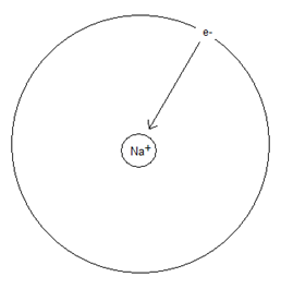
\(\newcommand{\avec}{\mathbf a}\) \(\newcommand{\bvec}{\mathbf b}\) \(\newcommand{\cvec}{\mathbf c}\) \(\newcommand{\dvec}{\mathbf d}\) \(\newcommand{\dtil}{\widetilde{\mathbf d}}\) \(\newcommand{\evec}{\mathbf e}\) \(\newcommand{\fvec}{\mathbf f}\) \(\newcommand{\nvec}{\mathbf n}\) \(\newcommand{\pvec}{\mathbf p}\) \(\newcommand{\qvec}{\mathbf q}\) \(\newcommand{\svec}{\mathbf s}\) \(\newcommand{\tvec}{\mathbf t}\) \(\newcommand{\uvec}{\mathbf u}\) \(\newcommand{\vvec}{\mathbf v}\) \(\newcommand{\wvec}{\mathbf w}\) \(\newcommand{\xvec}{\mathbf x}\) \(\newcommand{\yvec}{\mathbf y}\) \(\newcommand{\zvec}{\mathbf z}\) \(\newcommand{\rvec}{\mathbf r}\) \(\newcommand{\mvec}{\mathbf m}\) \(\newcommand{\zerovec}{\mathbf 0}\) \(\newcommand{\onevec}{\mathbf 1}\) \(\newcommand{\real}{\mathbb R}\) \(\newcommand{\twovec}[2]{\left[\begin{array}{r}#1 \\ #2 \end{array}\right]}\) \(\newcommand{\ctwovec}[2]{\left[\begin{array}{c}#1 \\ #2 \end{array}\right]}\) \(\newcommand{\threevec}[3]{\left[\begin{array}{r}#1 \\ #2 \\ #3 \end{array}\right]}\) \(\newcommand{\cthreevec}[3]{\left[\begin{array}{c}#1 \\ #2 \\ #3 \end{array}\right]}\) \(\newcommand{\fourvec}[4]{\left[\begin{array}{r}#1 \\ #2 \\ #3 \\ #4 \end{array}\right]}\) \(\newcommand{\cfourvec}[4]{\left[\begin{array}{c}#1 \\ #2 \\ #3 \\ #4 \end{array}\right]}\) \(\newcommand{\fivevec}[5]{\left[\begin{array}{r}#1 \\ #2 \\ #3 \\ #4 \\ #5 \\ \end{array}\right]}\) \(\newcommand{\cfivevec}[5]{\left[\begin{array}{c}#1 \\ #2 \\ #3 \\ #4 \\ #5 \\ \end{array}\right]}\) \(\newcommand{\mattwo}[4]{\left[\begin{array}{rr}#1 \amp #2 \\ #3 \amp #4 \\ \end{array}\right]}\) \(\newcommand{\laspan}[1]{\text{Span}\{#1\}}\) \(\newcommand{\bcal}{\cal B}\) \(\newcommand{\ccal}{\cal C}\) \(\newcommand{\scal}{\cal S}\) \(\newcommand{\wcal}{\cal W}\) \(\newcommand{\ecal}{\cal E}\) \(\newcommand{\coords}[2]{\left\{#1\right\}_{#2}}\) \(\newcommand{\gray}[1]{\color{gray}{#1}}\) \(\newcommand{\lgray}[1]{\color{lightgray}{#1}}\) \(\newcommand{\rank}{\operatorname{rank}}\) \(\newcommand{\row}{\text{Row}}\) \(\newcommand{\col}{\text{Col}}\) \(\renewcommand{\row}{\text{Row}}\) \(\newcommand{\nul}{\text{Nul}}\) \(\newcommand{\var}{\text{Var}}\) \(\newcommand{\corr}{\text{corr}}\) \(\newcommand{\len}[1]{\left|#1\right|}\) \(\newcommand{\bbar}{\overline{\bvec}}\) \(\newcommand{\bhat}{\widehat{\bvec}}\) \(\newcommand{\bperp}{\bvec^\perp}\) \(\newcommand{\xhat}{\widehat{\xvec}}\) \(\newcommand{\vhat}{\widehat{\vvec}}\) \(\newcommand{\uhat}{\widehat{\uvec}}\) \(\newcommand{\what}{\widehat{\wvec}}\) \(\newcommand{\Sighat}{\widehat{\Sigma}}\) \(\newcommand{\lt}{<}\) \(\newcommand{\gt}{>}\) \(\newcommand{\amp}{&}\) \(\definecolor{fillinmathshade}{gray}{0.9}\)To a very good approximation, the electronic spectra of highly excited atoms look a lot like the spectrum of hydrogen. These highly excited states of atoms are called “Rydberg States” and to a good approximation, the excited electron in a Rydberg state “feels” the nucleus of the atom as a point charge. As this occurs, the atom comes to be in a state that looks much like a state in a hydrogen-like atom, with a heavy nucleus that has \(a+1\) charge (the residual ion if the excited electron is removed).
In cases such as this, the energy levels of the excited electron can almost be treated using the Rydberg formula proposed by Balmer, and with the correct Rydberg constant (\(R_ {M}\) ) and nuclear charge. The formula does not work perfectly, but can be forced to fit the data by introducing a “fudge factor.”
Approximating a Hydrogen-like Atom
Scientists like to force the descriptions of real systems in terms of the limiting ideal cases with slight perturbations. In the case of real atoms, there are two common ways that this is typically done. One is to fudge the nuclear charge and the other is to fudge on the principle quantum number.
Shielding and Effective Nuclear Charge
One “fudges” the nuclear charge by noting that the excited electron will not “see” the inner core ion as a point charge with \(a +1\) charge. Instead, it will feel the full charge of the nucleus, but shielded by the electrons that remain in the ion. Thus, the effective nuclear charge (\(Z ^{*}\) ) can be used.
\[\tilde{\nu }=\left(Z^{*} \right)^{2} R_{M} \left(\dfrac{1}{n_{l}^{2} } -\dfrac{1}{n_{u}^{2} } \right)\nonumber \]
where \(Z ^{*}\), the effective nuclear charge, is defined by
\[Z ^{*} = Z – \sigma\nonumber \]
where \(\sigma\) is the shielding constant and is determined by adding the effects of each of the inner electrons. The trouble with this approach is that the degree of shielding is dependent on the excitation level of the excited electron. The shielding constant \(\sigma\) should reach a limiting value for highly excited Rydberg states of the atom.
Quantum Defect and the Effective Principal Quantum Number
Another approach is to “fudge” on the principle quantum number of the excited electron. The utility of using this method is that there is only one electron to treat, rather than a slew of electrons in the core ion, the shielding of each will be variable. In this method, the effective principal quantum number \(n^ {*}\) is defined as
\(n^ {*} = n – \delta\)
where \(\delta\) is the quantum defect. The quantum defect has the useful property that it reaches a constant value for electrons in atoms at high levels of excitation.
The ionization potential
The ionization potential of an atom I defined by the enthalpy change at 0 K for the following reaction
\[M \leftarrow M ^{+} + e ^{-} \qquad \Delta H = IP\nonumber \]
If one pictures ionization as a series of excitations of the electron to be removed through a set of Rydberg states, one can deduce the ionization potential of an atom. (This is how atomic spectroscopy is used to determine highly accurate ionization potentials.)
Using the effective principle quantum number \(n^ {*}\), the energy levels can be expressed as
\[\dfrac{E}{hc} =\dfrac{IP}{hc} -\dfrac{R_{M} }{(n^{*} )^{2} }\nonumber \]
Consider the Rydberg series in \(\ce{^{23}Na}\), the first few levels of which is given below. For \(\ce{Na}\), the Rydberg constant can be calculated
\[\begin{align*} R_{Na} =& \left(\dfrac{m_{Na} }{m_{e} +m_{Na}} \right)R_{\infty } \\[4pt] & =\left(\dfrac{3.81763 \times 10^{-26} kg}{9.109 \times 10^{-31} kg+3.81763 \times 10^{-26} kg} \right)\left(109737.316\; cm^{-1} \right) \\[4pt] &=109734.698\; cm^{-1} \end{align*} \]
Based on a guess of the ionization potential, an effective principle quantum number can be calculated for each level from
\[n^{*} =\sqrt{\dfrac{R_{Na} }{IP-E} }\nonumber \]
From \(n^ {*}\), one can calculate the quantum defect (\(\delta\)) and adjust the guess of the ionization potential until \(\Sigma\) becomes constant for large \(n\).
| \(IP =\) | \(41449.48 cm ^{-1}\) | \(R_ {Na} =\) | \(109734.7 \; cm ^{-1}\) | |
|---|---|---|---|---|
| Level | \(n\) | \(\delta\) | \(n*\) | Energy (\(cm ^{-1}\) ) |
| 3p | 3 | 0.883 | 2.117 | 16956.17 |
| 4p | 4 | 0.867 | 3.133 | 30266.99 |
| 5p | 5 | 0.862 | 4.138 | 35040.38 |
| 6p | 6 | 0.860 | 5.140 | 37296.32 |
| 7p | 7 | 0.858 | 6.142 | 38540.18 |
| 8p | 8 | 0.858 | 7.142 | 39298.35 |
| 9p | 9 | 0.857 | 8.143 | 39794.48 |
| 10p | 10 | 0.857 | 9.143 | 40136.80 |
| 11p | 11 | 0.857 | 10.143 | 40382.92 |
| 12p | 12 | 0.857 | 11.143 | 40565.78 |
| 13p | 13 | 0.857 | 12.143 | 40705.34 |
| 14p | 14 | 0.856 | 13.144 | 40814.27 |
| 15p | 15 | 0.856 | 14.144 | 40900.91 |
| 16p | 16 | 0.857 | 15.143 | 40970.97 |
| 17p | 17 | 0.857 | 16.143 | 41028.41 |
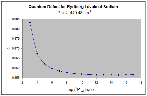
This method is extremely sensitive and can be used to determine very precise values of ionization potentials for atoms. The above result is 5.145 eV, whereas the literature value for the ionization potential of sodium is 5.139 eV (Webelements). The slightly large value determined from this data is a consequence of only using a limited number of excited levels, and not the highest energy levels, which behave most Rydberg-like. A close examination of the data actually reveals that there is some curvature to the \(\delta\) vs \(n\) curve at high values of \(n\). Since the curve is actually increasing at the larger values of \(n\), it is an indication that the guess for the ionization potential is slightly high – a fact that is consistent with the literature value!