5.7: Spectroscopy

The experimental determination of spectroscopic rotational constants provides a very precise set of data describing molecular structure. To see how experimental measurements inform the determination of molecular structure, let’s examine what is to be expected in the pure rotational spectrum of a molecule first.

Microwave Spectroscopy

The rotational selection rule in microwave absorption spectra is

\[\Delta \mathrm{J}=+1\nonumber \]

(Selection rules are discussed in more detail in a later section.) The pattern of lines predicted to be observed in a microwave spectrum (a pure rotational spectrum of a mole) can be derived by taking differences in rotational energy levels.

\[\begin{aligned} & \tilde{v}_{J}=F_{J+1}-F_{J} \\ F_{J+1}-F_{J}=& B(J+1)(J+2)-B J(J+1) \\ =& B\left(J^{2}+3 J+2\right)-B\left(J^{2}+J\right) \\ =& B\left(J^{2}+3 J+2-J^{2}-J\right) \\ =& B(2 J+2) \\ =& 2 B(J+1) \end{aligned}\nonumber \]

This suggests that a pure microwave spectrum should consist of a series of lines that are evenly spaces, the spacing between which is \(2 \mathrm{~B}\). It also suggests that a plot of the line frequency divided by \((\mathrm{J}+1)\) should yield a straight and horizontal line,

\[\dfrac{\tilde{v}_{J}}{(J+1)}=2 B\nonumber \]

The inclusion of distortion yields a slightly different conclusion.

\[\begin{aligned} F_{J+1}-F_{J} &=B(J+1)(J+2)-D[(J+1)(J+2)]^{2}-B J(J+1)+D[J(J+1)]^{2} \\ &=B\left(J^{2}+3 J+2-J^{2}-J\right)-D\left[\left(J^{2}+3 J+2\right)^{2}-\left(J^{2}+J\right)^{2}\right] \\ &=B(2 J+2)-D\left(J^{4}+6 J^{3}+13 J^{2}+12 J+4-J^{4}-2 J^{3}-J^{2}\right) \\ &= 2 B(J+1)-D\left(4 J^{3}+12 J^{2}+12 J+4\right) \\ &= 2 B(J+1)-4 D(J+1)^{3} \end{aligned}\nonumber \]

\[\dfrac{\tilde{v}_{J}}{(J+1)}=2 B-4 D(J+1)^{2}\nonumber \]

This suggests that a plot of \(\dfrac{\tilde{v}_{J}}{(J+1)}\) vs. \((J+1)^{2}\) should yield a straight line with slope -4D and intercept \(2 \mathrm{~B}\).

Consider the following set of data for the microwave spectrum of \(^{12} \mathrm{C}^{16} \mathrm{O}\) (Lovas & Krupenie, 1974).

A plot of \(\dfrac{\tilde{v}_{J}}{J+1}\) vs. \(J\) yields a plot as the following.

\(\mathrm{J}\)	\(\tilde{v}_{\mathrm{J}}\left(\mathrm{cm}^{-1}\right)\)
0	\(3.84503\)
1	\(7.68992\)
2	\(11.53451\)
3	\(15.37867\)
4	\(19.22223\)
5	\(23.06506\)
6	\(26.90701\)

Figure \(\PageIndex{1}\)

Clearly, this is not a horizontal line. The conclusion is that centrifugal distortion is not negligible for this molecule. Including distortion suggests that the plot that should be considered would involve \(\dfrac{\tilde{v}_{J}}{(J+1)}\) vs. \((\mathrm{J}+1)^{2}\). This yields the following:

Figure \(\PageIndex{2}\)

This does yield a straight line! From the fit, one calculates a B value of \(1.92253 \mathrm{~cm}^{-1}\) and a D value of \(0.00000612 \mathrm{~cm}^{-1}\).

Calculating a Bond Length from Spectroscopic Data

Spectroscopic data (and microwave data in particular) provides extremely high precision information from which bond lengths can be determined. Based on the above data and the masses of carbon-12 (12.00000 amu) and oxygen-16 (15.99491463 amu) (Rosman & Taylor, 1998) a reduced mass for \({ }^{12} \mathrm{C}^{16} \mathrm{O}\) can be calculated as

\[\mu=\dfrac{m_{C} m_{O}}{m_{C}+m_{O}}=6.85621 \mathrm{amu}=1.1385 \times 10^{-26} \mathrm{~kg}\nonumber \]

Recalling the expression for the rotational constant B

\[B=\dfrac{h}{8 \pi^{2} c \mu r^{2}}\nonumber \]

The bond length is given by

\[r=\sqrt{\dfrac{h}{8 \pi^{2} c \mu B}}\nonumber \]

Using the data from above, one calculates a bond length for CO to be \(r=1.1312 \mathring{\mathrm{A}}\). This value is actually the average value of the bond length in the \(v=0\) level. The literature value for the equilibrium bond length (the bond length at the potential minimum) is given by \(r_{e}=1.128323 \mathring{\mathrm{A}}\) (Bunker, 1970) which is slightly shorter (as is to be expected.) The extrapolation of data to determine values at the potential minimum is discussed in a later section.

Rotation-Vibration Spectroscopy

Each vibrational level in a molecule will have a whole stack of rotational energy levels. As such, vibrational transitions will also show rotational fine structure. This fine structure can be analyzed to determine very precise values for molecular structure in much the same ways microwave data for the pure rotational spectrum can be. One method for analyzing this data is that of combination differences although direct fitting of the data will give better results mathematically. Before beginning a discussion of combination differences, however, it is necessary to discuss selection rules.

Selection Rules and Branch Structure

Selection rules are determined for spectroscopic transitions as those transitions for which the transition moment integral does not vanish. This is because the observed intensities of spectroscopic transitions are proportional to the squared magnitude of the transition moment. The transition moment integral is given by

\[\int\left(\psi^{\prime}\right)^{*} \vec{\mu}\left(\psi^{\prime \prime}\right) d \tau\nonumber \]

and so the intensities of transitions are given by

\[\text { Int. } \propto\left|\int\left(\psi^{\prime}\right)^{*} \vec{\mu}\left(\psi^{\prime \prime}\right) d \tau\right|^{2}\nonumber \]

where a single prime (’) indicates the upper state of the transition and a double prime (") indicates the lower state. The operator \(\vec{\mu}\) corresponds to the change in the electric dipole moment of the molecule as it undergoes a transition from a state described by \(\psi\) " to one described by \(\psi\) ’. Other operators may be used in this expression (magnetic dipole, electric quadrupole, etc.) but these lead to significantly weaker transitions (by a factor of \(10^{6}\) or more!) When the electric dipole operator is used, the transitions for which the transition moment is not zero are said to be allowed transitions, while all others are said to be forbidden transitions by electric dipole selection rules. Since other types of transitions are so weak by comparison, a transition that is said to be allowed or forbidden is assumed to mean by electric dipole selection rules unless specifically stated otherwise.

The selection rules for vibrational transitions are

\[\Delta \mathrm{v}=\pm 1\nonumber \]

For closed-shell molecules (molecules where all of the electrons are paired), the rotational selection rules are

\[\Delta \mathrm{J}=\pm 1\nonumber \]

\(\Delta \mathrm{J}=0\) is possible for some open-shell molecules, but his topic will be discussed in more detail in Chapter 7.

The rotational fine structure of a transition can be separated into branches according to the specific change in the rotational quantum number \(J\).

\(\mathbf{\Delta J}\)
\(+1\)	R-branch
0	Q-branch
\(-1\)	P-branch

In Raman spectroscopy (which is an inelastic light scattering process rather than the direct absorption or emission of a photon, and thus follows different selection rules) O- and S-Branches can be observed with \(\Delta \mathrm{J}=-2\) and \(+2\) respectively.

The spectrum of possible branches and transitions that can be observed for all possible molecules can be quite daunting (and take an entire graduate level course in molecular spectroscopy just to scratch the surface!) For the purposes of this discussion, we will limit ourselves for the time being to just closed-shell molecules for which P- and R-branches can be observed.

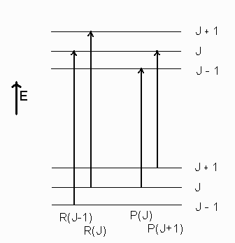
Consider the following energy level diagram depicting the rotational energy levels in two different states. The diagram shows the expected branch structure for a closed shell molecule. Notice that the transition lines get longer with increasing \(\mathrm{J}\) in the R-branch, but shorter with increasing \(\mathrm{J}\) in the P-branch. The largest difference in transition energy is for successive lines in the spectrum is that between the \(\mathrm{R}_{0}\) and \(\mathrm{P}_{1}\) lines. The band origin \(\left(\tilde{v}_{0}\right)\) will lie between these two lines, and is at the energy difference between the \(J^{\prime}=0\) and \(J\) " \(=0\), the two non-rotating levels in the two vibrational levels. Also notice that the rotational energy spacings in the upper state are smaller than those in the lower state. This is do to a smaller \(\mathrm{B}\) value in the upper state \((\mathrm{v}=\) 1), which has a larger average bond length than the \(v=0\) level.

Energy Level Diagram

Figure \(\PageIndex{3}\)

Combination Differences

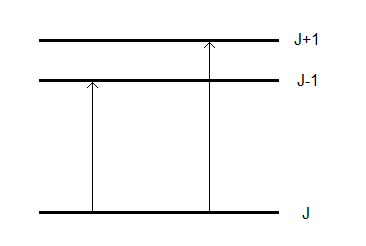
Consider the following partial energy level diagram:

Figure \(\PageIndex{4}\)

It is clear that since the \(\mathrm{R}(\mathrm{J})\) and \(\mathrm{P}(\mathrm{J})\) transitions share a common lower rotational level \(\left(F_{J}\right)\), the energy difference between the \(R(J)\) and \(P(J)\) transitions gives the energy difference between the \(\mathrm{F}_{\mathrm{J}+1}\) and \(\mathrm{F}_{\mathrm{J}-1}\) in the upper state of the transition. Similarly, the difference between \(F_{J+1}\) and \(F_{J-1}\) in the lower state is given by \(R(J-1)-P(J+1)\). Thus, by taking differences of transition energies in the proper combination, dependence on one of the states can be eliminated. Also, the difference \(\Delta_{2} \mathrm{~F}(\mathrm{~J})\) can be found. This difference is defined by:

\[\Delta_{2} \mathrm{~F}(\mathrm{~J}) \equiv \mathrm{F}_{\mathrm{J}+1}-\mathrm{F}_{\mathrm{J}-1}\nonumber \]

Using the rigid rotator model,

\[F_{J}=B J(J+1)\nonumber \]

an expression for \(\Delta_{2} F(J)\) can be easily derived:

\[\begin{aligned} \Delta_{2} \mathrm{~F}(\mathrm{~J}) &=\mathrm{B}(\mathrm{J}+1)(\mathrm{J}+2)-\mathrm{B}(\mathrm{J}-1)(\mathrm{J}) \\ &=\mathrm{B}\left(\mathrm{J}^{2}+3 \mathrm{~J}+2\right)-\mathrm{B}\left(\mathrm{J}^{2}-\mathrm{J}\right) \\ &=\mathrm{B}(4 \mathrm{~J}+2) \\ &=4 \mathrm{~B}\left(J+\dfrac{1}{2}\right) \end{aligned}\nonumber \]

Thus the value of \(\Delta_{2} \mathrm{~F}(\mathrm{~J})\) that can be found for either the upper or lower states by combination differences from the energies of the spectral lines, can be used to find the spectroscopic constant B.

\[\dfrac{\Delta_{2} F(J)}{\left(J+\dfrac{1}{2}\right)}=4 B\nonumber \]

And the \(\Delta_{2} \mathrm{~F}(\mathrm{~J})\) values are determined by the combination differences

\[\begin{gathered} \Delta_{2} F^{\prime}(J)=R(J)-P(J) \\ \Delta_{2} F^{\prime \prime}(J)=R(J-1)-P(J+1) \end{gathered}\nonumber \]

were the single prime (") refers to the upper state and the double prime (") refers to the lower state.

For most molecules, the rotational distortion constants are not negligible. In this case, the rotational term values are given by

\[\mathrm{F}(\mathrm{J})=\mathrm{BJ}(\mathrm{J}+1)-\mathrm{DJ}^{2}(\mathrm{~J}+1)^{2}+\mathrm{HJ}^{3}(\mathrm{~J}+1)^{3}+\ldots\nonumber \]

Neglecting terms of higher order than \(\mathrm{DJ}^{2}(\mathrm{~J}+1)^{2}\) (since these terms are small for most molecules) the combination differences relationship can be derived as

\[\begin{aligned} \Delta_{2} \mathrm{~F}(\mathrm{~J}) &=\mathrm{B}(\mathrm{J}+1)(\mathrm{J}+2)-\mathrm{D}(\mathrm{J}+1)^{2}(\mathrm{~J}+2)^{2}-\mathrm{B}(\mathrm{J}-1)(\mathrm{J})+\mathrm{D}(\mathrm{J}-1)^{2}(\mathrm{~J})^{2} \\ &=\mathrm{B}\left[\left(\mathrm{J}^{2}+3 \mathrm{~J}+2\right)-\left(\mathrm{J}^{2}-\mathrm{J}\right)\right]-\mathrm{D}\left[\left(\mathrm{J}^{2}+2 \mathrm{~J}+1\right)\left(\mathrm{J}^{2}+4 \mathrm{~J}+4\right)-\left(\mathrm{J}^{2}-2 \mathrm{~J}+1\right) \mathrm{J}^{2}\right] \\ &=\mathrm{B}(4 \mathrm{~J}+2)-\mathrm{D}\left(\mathrm{J}^{4}+4 \mathrm{~J}^{3}+4 \mathrm{~J}^{2}+2 \mathrm{~J}^{3}+8 \mathrm{~J}^{2}+8 \mathrm{~J}+\mathrm{J}^{2}+4 \mathrm{~J}+4-\mathrm{J}^{4}+2 \mathrm{~J}^{3}-\mathrm{J}^{2}\right) \\ &=4 \mathrm{~B}\left(J+\dfrac{1}{2}\right)-\mathrm{D}\left(8 \mathrm{~J}^{3}+12 \mathrm{~J}^{2}+12 \mathrm{~J}+4\right) \\ &=4 \mathrm{~B}\left(J+\dfrac{1}{2}\right)-8 \mathrm{D}\left(\mathrm{J}^{3}+\dfrac{3}{2} \mathrm{~J}^{2}+\dfrac{3}{2} \mathrm{~J}+\dfrac{1}{2}\right) \end{aligned}\nonumber \]

It would be convenient if the term involving \(\mathrm{D}\) could be factored. Recognizing that

\[\left(J+\dfrac{1}{2}\right)^{3}=\mathrm{J}^{3}+\dfrac{3}{2} \mathrm{~J}^{2}+\dfrac{3}{4} \mathrm{~J}+\dfrac{1}{8}\nonumber \]

the "cube" can be "completed" by

\[\begin{aligned} \Delta_{2} \mathrm{~F}(\mathrm{~J}) &=4 \mathrm{~B}\left(J+\dfrac{1}{2}\right)-8 \mathrm{D}\left(\mathrm{J}^{3}+\dfrac{3}{2} \mathrm{~J}^{2}+\dfrac{3}{4} \mathrm{~J}+\dfrac{1}{8}+\dfrac{3}{4} \mathrm{~J}+\dfrac{3}{8}\right) \\ &=4 \mathrm{~B}\left(J+\dfrac{1}{2}\right)-8 \mathrm{D}\left(J+\dfrac{1}{2}\right)^{3}-8 \mathrm{D}(\dfrac{3}{4} \mathrm{~J}+\dfrac{3}{8}) \\ &=4 \mathrm{~B}\left(J+\dfrac{1}{2}\right)-8 \mathrm{D}\left(J+\dfrac{1}{2}\right)^{3}-\mathrm{D}(6 \mathrm{~J}+3) \\ &=4 \mathrm{~B}\left(J+\dfrac{1}{2}\right)-8 \mathrm{D}\left(J+\dfrac{1}{2}\right)^{3}-6 \mathrm{D}\left(J+\dfrac{1}{2}\right) \\ &=[4 \mathrm{~B}-6 \mathrm{D}]\left(J+\dfrac{1}{2}\right)-8 \mathrm{D}\left(J+\dfrac{1}{2}\right)^{3} \end{aligned}\nonumber \]

And by dividing through by \(\left(J+\dfrac{1}{2}\right)\)

\[\dfrac{\Delta_{2} F(J)}{\left(J+\dfrac{1}{2}\right)}=[4 \mathrm{~B}-6 \mathrm{D}]-8 \mathrm{D}\left(J+\dfrac{1}{2}\right)^{2}\nonumber \]

So using the spectral data, a plot of

\[\begin{gathered} \dfrac{\mathrm{R}(\mathrm{J})-\mathrm{P}(\mathrm{J})}{\left(J+\dfrac{1}{2}\right)} \text { vs. }\left(J+\dfrac{1}{2}\right)^{2} \\ \text { or } \\ \dfrac{\mathrm{R}(\mathrm{J}-1)-\mathrm{P}(\mathrm{J}+1)}{\left(J+\dfrac{1}{2}\right)} \text { vs. }\left(J+\dfrac{1}{2}\right)^{2} \end{gathered}\nonumber \]

should yield straight lines with slopes of \(8 \mathrm{D}\) and an intercept of \((4 \mathrm{~B}-6 \mathrm{D})\) for the upper and lower states respectively.

Additional Spectroscopic Constants

Since each vibrational level has a different average bond length (increasing with increasing vibrational quantum number for a well-behaved electronic state,) the rotational constant has a dependence on the vibrational quantum number \(\mathrm{v}\).

\[B_{v}=B_{e}-\alpha_{e}\left(v+\dfrac{1}{2}\right)+\gamma_{e}\left(v+\dfrac{1}{2}\right)^{2}+\ldots\nonumber \]

where \(B_{\mathrm{e}}\) is the equilibrium value of the rotational constant (and the constant from which \(\mathrm{r}_{\mathrm{e}}\) is derived), \(\alpha_{\mathrm{e}}\) and \(\gamma_{\mathrm{e}}\) are constants that describe how rotation and vibration are coupled in a molecule. Usually this power series in \(\left(\mathrm{v}+\dfrac{1}{2}\right)\) can be truncated at the \(\alpha_{\mathrm{e}}\) term (unless data for a great many vibrational levels are known.)

Similarly, the distortional term can be expanded in a power series in \(\left(\mathrm{v}+\dfrac{1}{2}\right)\).

\[D_{v}=D_{e}-\beta_{e}\left(v+\dfrac{1}{2}\right)+\ldots\nonumber \]

For most molecules, \(\beta_{\mathrm{e}}\) is not determined within experimental uncertainty unless a great many vibrational levels have been included in the fit.

A typical methodology would be to determine \(\mathrm{B}_{\mathrm{v}}\) for all of the vibrational levels for which data exists. (A single vibration-rotation band analysis provides two values, one for the upper state and one for the lower state.) Then the \(B_{\mathrm{v}}\) values are fit to the functional form given by

\[B_{v}=B_{e}-\alpha_{e}\left(v+\dfrac{1}{2}\right)+\gamma_{e}\left(v+\dfrac{1}{2}\right)^{2}+\ldots\nonumber \]

truncating the power series so as to include the minimum number of adjustable parameters as are needed to yield a good fit to the data. This process yields a value for \(\mathrm{B}_{\mathrm{e}}\) which can then be used to calculate \(r_{e}\). These values can then be compared to those found in the literature (if such a value has been measured) or reported in the literature if it has not yet been measured! A similar approach is used for the distortional term(s).

Line Intensity in Rotational Structure

One element that we have not discussed in the subject of rotational spectroscopy (or the rotational fine structure in vibration-rotation spectroscopy) is the intensities of the spectral lines. The intensity will be determined by two factors: 1) the population of the originating state (lower state in absorption and upper state in emission spectra) which is well described for a thermalized sample by a Maxwell-Boltzmann distribution, and 2) the line strength, which is determined by the quantum mechanical relationship between the upper and lower states of the transition.

The Maxwell-Boltzmann Distribution

The Maxwell-Boltzmann distribution of energy level populations will be achieved by any system that is in thermal equilibrium (usually implying that a sufficient number of molecular collisions occur for a gas phase sample, or that all of the parts of a sample are in thermal contact with one another in condensed phase samples) to ensure thermal uniformity throughout the sample. The distribution is given by the following expression:

\[\dfrac{N_{i}}{N_{t o t}}=\dfrac{d_{i} e^{-E_{i} / k T}}{q}\nonumber \]

where \(\frac{N_{i} }{N_{\text {tot }}}\) is the fraction of molecules in the \(i^{\text {th }}\) quantum state, that has and energy given by \(E_{i}\) and a degeneracy given by \(d_{i}\). The term \(k T\) is the Boltzmann constant times the temperature on an absolute scale. The denominator, \(q\), is a partition function, which is part of a normalization factor. The partition function is given by

\[q=\sum_{i} d_{i} e^{-E_{i} / k T}\nonumber \]

In the case of rotational energy levels for closed-shell molecules, the subscript I can be replaced by the rotational quantum number \(\mathrm{J}\).

\[q_{r o t}=\sum_{J} d_{J} e^{-E_{J} / k T}\nonumber \]

In this expression, the rotational energy level degeneracies are always given by \((2J+1)\) and the rotational energy levels (if treated as rigid rotor levels) are given by \(hcBJ(J+1)\). Thus the expression for the rotational partition function, qrot, is given by

\[q_{r o t}=\sum_{J}(2 J+1) e^{-h c B J(J+1) / k T}\nonumber \]

It is handy to note that \(\frac{hc}{kT}\) has a value of approximately \(206 \mathrm{~cm}^{-1}\) at room temperature. When the energy \(E_{i}\) exceeds approximately \(10 \cdot \mathrm{kT}\), the exponential term becomes negligibly small.

Focusing on the numerator of the Maxwell-Boltzmann expression, it is clear that the effect of increasing \(\mathrm{J}\) is mixed in the expression. As \(\mathrm{J}\) increases, the degeneracy increases (having the effect of increased fractional population in the level) but also the exponential term gets smaller due to the higher energy (having the effect of a decreased fractional population in the energy level.) A plot of factional population as a function of \(\mathrm{J}\) (for \(\mathrm{HCl}\) at \(298 \mathrm{~K}\) ) is shown below.

Figure \(\PageIndex{5}\)

Note that at low values of \(\mathrm{J}\), the fractional population increases with increasing \(\mathrm{J}\), to a point. Eventually, the exponential term takes over and the population is extinguished. The \(J\) value \(\left(\mathrm{J}_{\max }\right)\) at which this changeover occurs is a function of the rotational constant \(\mathrm{B}\) and the temperature, and can be determined by solving the following expression for \(\mathrm{J}\).

\[\dfrac{d}{d J}(2 J+1) e^{\frac{-h c B J(J+1)}{kT}}=0\nonumber \]

The result is

\[J_{\max }=\sqrt{\dfrac{k T}{2 B h c}}-\dfrac{1}{2}\nonumber \]

The intensity pattern is plainly visible in the rotation-vibration spectrum of \(HCl\). A simulated spectrum of the 1-0 band of \(H^{35} Cl\) is shown below, clearly showing the P- and R-branch structure, and the large gap between where the band origin can be found.

Figure \(\PageIndex{6}\)

Line Strength Considerations

The second major consideration in spectral line intensity is the line strength. This is determined by the squared magnitude of the transition moment integral.

\[\text { Int. } \propto\left|\int\left(\psi^{\prime}\right)^{*} \vec{\mu}\left(\psi^{\prime \prime}\right) d \tau\right|^{2}\nonumber \]

The rotational contribution, often called the rotational line strength, to this expression is a HönlLondon factor. For closed shell diatomic molecules, the Hönl-London factors are given by

\[\begin{array}{ll} \mathrm{S}_{\mathrm{J}}=\mathrm{J}+1 & \text { (for R-branch lines) } \\ \mathrm{S}_{\mathrm{J}}=\mathrm{J} & \text { (for P-branch lines) } \end{array}\nonumber \]

A good way to think of these expressions is to view them as branching ratios. They indicate the relative fraction of molecules in a given level that will undergo an R-branch transition compared to what fraction will undergo a P-branch transition. The molecules the lower state must "decide" to undergo either an R-branch transition or a P-branch transition. The relative fraction of each type of "decision" is the branching ratio.

Figure \(\PageIndex{7}\)

Notice that the sum of these two expressions gives the total degeneracy of the rotational level. Given this relationship, it should be clear that the fractions of molecules undergoing each type of transition are given by

\[F_{R}=\dfrac{J+1}{2 J+1} \quad \text { and } \quad F_{P}=\dfrac{J}{2 J+1}\nonumber \]

For open shell molecules, the expressions can be quite a bit more complex, but that is a topic for a more detailed course on molecular spectroscopy. However, some of the details of rotational structure of open shell molecules will be discussed in Chapter 8, as the electronic portion of the molecular wavefunction can affect the rotational structure profoundly.