
1.5: On Superposition and the Weirdness of Quantum Mechanics
- Page ID
- 420469

\( \newcommand{\vecs}[1]{\overset { \scriptstyle \rightharpoonup} {\mathbf{#1}} } \)
\( \newcommand{\vecd}[1]{\overset{-\!-\!\rightharpoonup}{\vphantom{a}\smash {#1}}} \)
\( \newcommand{\id}{\mathrm{id}}\) \( \newcommand{\Span}{\mathrm{span}}\)
( \newcommand{\kernel}{\mathrm{null}\,}\) \( \newcommand{\range}{\mathrm{range}\,}\)
\( \newcommand{\RealPart}{\mathrm{Re}}\) \( \newcommand{\ImaginaryPart}{\mathrm{Im}}\)
\( \newcommand{\Argument}{\mathrm{Arg}}\) \( \newcommand{\norm}[1]{\| #1 \|}\)
\( \newcommand{\inner}[2]{\langle #1, #2 \rangle}\)
\( \newcommand{\Span}{\mathrm{span}}\)
\( \newcommand{\id}{\mathrm{id}}\)
\( \newcommand{\Span}{\mathrm{span}}\)
\( \newcommand{\kernel}{\mathrm{null}\,}\)
\( \newcommand{\range}{\mathrm{range}\,}\)
\( \newcommand{\RealPart}{\mathrm{Re}}\)
\( \newcommand{\ImaginaryPart}{\mathrm{Im}}\)
\( \newcommand{\Argument}{\mathrm{Arg}}\)
\( \newcommand{\norm}[1]{\| #1 \|}\)
\( \newcommand{\inner}[2]{\langle #1, #2 \rangle}\)
\( \newcommand{\Span}{\mathrm{span}}\) \( \newcommand{\AA}{\unicode[.8,0]{x212B}}\)
\( \newcommand{\vectorA}[1]{\vec{#1}} % arrow\)
\( \newcommand{\vectorAt}[1]{\vec{\text{#1}}} % arrow\)
\( \newcommand{\vectorB}[1]{\overset { \scriptstyle \rightharpoonup} {\mathbf{#1}} } \)
\( \newcommand{\vectorC}[1]{\textbf{#1}} \)
\( \newcommand{\vectorD}[1]{\overrightarrow{#1}} \)
\( \newcommand{\vectorDt}[1]{\overrightarrow{\text{#1}}} \)
\( \newcommand{\vectE}[1]{\overset{-\!-\!\rightharpoonup}{\vphantom{a}\smash{\mathbf {#1}}}} \)
\( \newcommand{\vecs}[1]{\overset { \scriptstyle \rightharpoonup} {\mathbf{#1}} } \)
\( \newcommand{\vecd}[1]{\overset{-\!-\!\rightharpoonup}{\vphantom{a}\smash {#1}}} \)
\(\newcommand{\avec}{\mathbf a}\) \(\newcommand{\bvec}{\mathbf b}\) \(\newcommand{\cvec}{\mathbf c}\) \(\newcommand{\dvec}{\mathbf d}\) \(\newcommand{\dtil}{\widetilde{\mathbf d}}\) \(\newcommand{\evec}{\mathbf e}\) \(\newcommand{\fvec}{\mathbf f}\) \(\newcommand{\nvec}{\mathbf n}\) \(\newcommand{\pvec}{\mathbf p}\) \(\newcommand{\qvec}{\mathbf q}\) \(\newcommand{\svec}{\mathbf s}\) \(\newcommand{\tvec}{\mathbf t}\) \(\newcommand{\uvec}{\mathbf u}\) \(\newcommand{\vvec}{\mathbf v}\) \(\newcommand{\wvec}{\mathbf w}\) \(\newcommand{\xvec}{\mathbf x}\) \(\newcommand{\yvec}{\mathbf y}\) \(\newcommand{\zvec}{\mathbf z}\) \(\newcommand{\rvec}{\mathbf r}\) \(\newcommand{\mvec}{\mathbf m}\) \(\newcommand{\zerovec}{\mathbf 0}\) \(\newcommand{\onevec}{\mathbf 1}\) \(\newcommand{\real}{\mathbb R}\) \(\newcommand{\twovec}[2]{\left[\begin{array}{r}#1 \\ #2 \end{array}\right]}\) \(\newcommand{\ctwovec}[2]{\left[\begin{array}{c}#1 \\ #2 \end{array}\right]}\) \(\newcommand{\threevec}[3]{\left[\begin{array}{r}#1 \\ #2 \\ #3 \end{array}\right]}\) \(\newcommand{\cthreevec}[3]{\left[\begin{array}{c}#1 \\ #2 \\ #3 \end{array}\right]}\) \(\newcommand{\fourvec}[4]{\left[\begin{array}{r}#1 \\ #2 \\ #3 \\ #4 \end{array}\right]}\) \(\newcommand{\cfourvec}[4]{\left[\begin{array}{c}#1 \\ #2 \\ #3 \\ #4 \end{array}\right]}\) \(\newcommand{\fivevec}[5]{\left[\begin{array}{r}#1 \\ #2 \\ #3 \\ #4 \\ #5 \\ \end{array}\right]}\) \(\newcommand{\cfivevec}[5]{\left[\begin{array}{c}#1 \\ #2 \\ #3 \\ #4 \\ #5 \\ \end{array}\right]}\) \(\newcommand{\mattwo}[4]{\left[\begin{array}{rr}#1 \amp #2 \\ #3 \amp #4 \\ \end{array}\right]}\) \(\newcommand{\laspan}[1]{\text{Span}\{#1\}}\) \(\newcommand{\bcal}{\cal B}\) \(\newcommand{\ccal}{\cal C}\) \(\newcommand{\scal}{\cal S}\) \(\newcommand{\wcal}{\cal W}\) \(\newcommand{\ecal}{\cal E}\) \(\newcommand{\coords}[2]{\left\{#1\right\}_{#2}}\) \(\newcommand{\gray}[1]{\color{gray}{#1}}\) \(\newcommand{\lgray}[1]{\color{lightgray}{#1}}\) \(\newcommand{\rank}{\operatorname{rank}}\) \(\newcommand{\row}{\text{Row}}\) \(\newcommand{\col}{\text{Col}}\) \(\renewcommand{\row}{\text{Row}}\) \(\newcommand{\nul}{\text{Nul}}\) \(\newcommand{\var}{\text{Var}}\) \(\newcommand{\corr}{\text{corr}}\) \(\newcommand{\len}[1]{\left|#1\right|}\) \(\newcommand{\bbar}{\overline{\bvec}}\) \(\newcommand{\bhat}{\widehat{\bvec}}\) \(\newcommand{\bperp}{\bvec^\perp}\) \(\newcommand{\xhat}{\widehat{\xvec}}\) \(\newcommand{\vhat}{\widehat{\vvec}}\) \(\newcommand{\uhat}{\widehat{\uvec}}\) \(\newcommand{\what}{\widehat{\wvec}}\) \(\newcommand{\Sighat}{\widehat{\Sigma}}\) \(\newcommand{\lt}{<}\) \(\newcommand{\gt}{>}\) \(\newcommand{\amp}{&}\) \(\definecolor{fillinmathshade}{gray}{0.9}\)In order to better appreciate the fascinating (and sometimes shocking!) results of the quantum world, let’s consider some measurable properties of electrons. Consider in particular two specific properties they exhibit. It doesn’t really matter what these properties actually are, but it does matter that there are only two possible outcomes when measuring these properties. For the purposes of this discussion, we can call these properties Latin and Greek, and the two measurable values of these properties are X or Y (for Latin) and a or b (for Greek.)
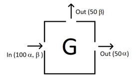
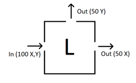
For the purposes of this discussion, let us assume that we can build a perfect sorting box for each property. For example, we can build a “Latin” box that will direct electrons though an aperture based on whether the electron is detected to have the value X, and a different aperture if the electron is found to have the value Y. Such a box would work as follows:

Similarly, we can build a “Greek” box that will sort in the same manner, except according to the measured value of the Greek property:
Are the Properties Repeatable?
We can use these boxes to test whether or not the measured values of the Greek and Latin properties are repeatable. In order to do this, consider directing the X aperture output of a Latin box into a second Latin box. If the measured value of the property is repeatable, we would expect all of the electrons to exit the second Latin box through the X aperture. Pictorially, the second box would look as follows

demonstrating that the property is indeed repeatable. The same behavior is observed using the Greek box, in that previously measured a electrons will always exit the a aperture of the Greek box.
Are the Properties Correlated?
A reasonable question to ask is whether or not the properties are correlated. An example of this correlation would be observed if previously measured X electrons were more likely to be measured as a electrons afterward. The apparatus for testing for this kind of correlation might look as follows:

As is suggested in the diagram, the outcome of the Greek measurement does not show any preference for a or b for previously measured X electrons. The outcome for measuring a electrons with a Latin box is similar, in that half of the electrons exit the X aperture and half exit the Y aperture. The conclusion, therefore, would be that the Latin and Greek properties are not correlated.
Now, suppose we try a third variation and create a three-box experiment. In this experiment, we will use a Latin box to select the X electrons out of an initial random stream of electrons. These will then run through a Greek box. We will then take the a aperture output of the Greek box and run that through a Latin box. The box arrangement for this experiment would look as follows:


What do you expect for the percentages of electrons leaving the Latin box apertures? As it turns out, half of the a electrons leaving the Greek box will exit the X aperture and half will exit the Y aperture. As crazy as it seems, it appears that measuring the Greek property made the electrons “forget” that they were previously measured to be X electrons!
This has an important implication about the nature of these sorting boxes. It implies that it would be impossible to build a compound box (a larger box constructed for Latin and Greek boxes) that would simultaneously sort electrons by both Latin and Greek properties. In other words, the following device would not work:
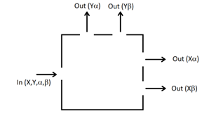
The reason this box will not work is that the electrons do not behave as though they carry definite values of Latin or Greek properties. Rather, these properties have to be determined at the time of measurement. The result is contrary to the behavior of any particle that is well-described by Newtonian physics!
To help illustrate this, consider randomizing the state of a quarter ($0.25) by flipping it. We know that it will land as either heads or tails. But we can also imagine it landing with the head (or tail) upright or upside down. The coin can, in effect, land in one of four states. For convenience, let’s label them as HU, TU, HD, and TD (H/T for heads or tails, and U/D for up or down.

For a classical object, like a coin, we expect all of the physical properties to persist. For example, if we flip the coin, and then measure in order, heads or tails, up or down, and then heads or tails, we expect the results of the first and third measurements to yield the same result.
But in the case of the electron, measuring the Greek property seemed to cause the electron to completely forget what was measured about the Latin property. This leads us to the conclusion that there is not an internal property that determines the outcome of the measurement of that Latin property – ant least not one that can survive the measurement of the Greek property.
Do the Properties Interfere with One Another?
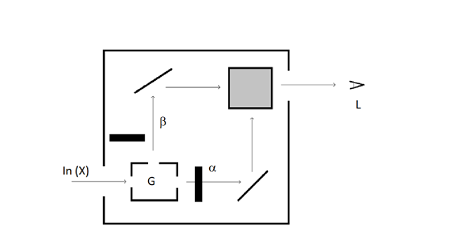
While it is true that electrons can not be definitively sorted simultaneously by Latin and Greek properties due to the lack of persistence of the measured outcomes when mixing boxes, one might ask if measuring one outcome interferes with the measurement of a second. Consier a new type of compound box, into which we will introduce two new devices: mirrors, and what we can consider a “combining” box. The role of the mirrors is simply to redirect a beam, but they will not alter the beam in any other way that its direction of travel. Similarly, the “combining” box will only collect the beams and cause them to travel in the same direction.
The box will be designed to accept the input of a beam of electrons previously selected as X electrons. It will then sort by Latin or Greek properties, redirect and combine the beams and then measure for either Latin or Greek properties at the exit aperture. Such a compound device might look as follows:

Such a device could be configured for four different interesting experiments. These experiments are described below:
- Sort the X electrons using a Latin box, and measure the Latin property at the exit
- Sort the X electrons using a Latin box, and measure the Greek property at the exit
- Sort the X electrons using a Greek box, and measure the Greek property at the exit
- Sort the X electrons using a Greek box, and measure the Latin property at the exit
The results of these experiments are summarized in the table below:
| Experiment | Input | Sorter | Detector | Result? |
|---|---|---|---|---|
| I | 100% X | Latin | Latin | 100% X |
| II | 100% X | Latin | Greek | 50% a, 50% b |
| III | 100% X | Greek | Greek | 50% a, 50% b |
| IV | 100% X | Greek | Latin | ??? |
Let’s consider the results individually.
Experiment I

The results of this experiment are not surprising based on the results of the previous sections. Consider the path that the electrons will take as they pass through the apparatus. All of the X electrons incident on the box will be sorted to exit the X aperture of the Latin box and travel to the detector where they will again be measured as X electrons. This is the expected result because the property is measured to be repeatable by successive boxes of the same type.
Experiment II

Again, the result is not too surprising. We expect all of the electrons to exit the “sorting” box along the X pathway. And since the Greek property is not correlated to the Latin property, when measured at the Greek detector, we expect 50% a and 50% b electrons to be detected.
Experiment III

In this experiment, things are getting to be more interesting, as we have to consider electrons exiting the “sorting” box along both the a and b paths, each accounting for half of the initial X electrons. Of the electrons that travel along the a path (which is expected to be 50% of the incident X electrons), we expect them all to be measured as a electrons. Similarly for those electrons which follow the b path, we expect them to be detected as b electrons at the detector.
Experiment IV

In this configuration, one might expect half of the incident X electrons to exit the sorter along the a path, and when detected, half will be X, and half will be Y. Similarly for those electrons that travel along the b path, half will be detected as X and half will be detected as Y. This would result in a total of 50% X and 50% Y. And this result seems perfectly reasonable based on our initial results.
But the quantum world has a huge surprise for us. In this experiment 100% of the electrons are detected as X electrons! How is this possible? It seems to completely contradict the notion that measuring the Greek property causes the electron to lose its Latin identity. On its face, this result seems completely absurd and impossible, but the behavior is observed on electrons, photons, and even large molecules such as buckyballs (\(C_{60}\) molecules)!
Further Developments
Let’s consider a new apparatus in which beam stoppers can be introduced to block the individual a and b paths inside the box. This setup might look something like what is depicted in the diagram below.
This suggests four new experiments, the designs and results of which are listed in the table below:
| Experiment | a-path | b-path | ||
|---|---|---|---|---|
| A | open | open | 100% X | 0% Y |
| B | open | blocked | 25% X | 25% Y |
| C | blocked | open | 25% X | 25% Y |
| D | blocked | blocked | 0% X | 0% Y |
These results allow us to draw some important (but classically troubling) conclusions about the pathway the electrons are taking through the box.
Do they take the a-path or the b-path?
If the a-path is open (experiments A and B) we detect electrons at the exit, but the intensity is reduced by 50% if the b-path is blocked (Experiment B). This result is consistent with the interpretation that half of the electrons take the a-path and half take the b-path, and also is consistent with what we expect based on previous experiments. However, because we now see a split of both X and Y electrons detected at the exit rather than 100% X, we have to conclude that they electrons are not simply taking the b-path. And further, we can conclude that they are not simply taking the a-path given the results of experiment C!
Are they somehow taking both paths?
It may seem like a silly question, but if they were taking both paths, blocking one of the paths would result in a half electron being detected at the exit if the incident beam was slowed sufficiently – and that never happens! Electrons are always detected whole and intact. So we can conclude that the electrons are also not magically splitting into half with each half taking one of the paths.
Is it possible they take neither path?
The results of experiment D for us to reject this possibility as well, since blocking both paths eliminates any detected signals at the exit. They must be somehow using the pathways but without picking one or the other, and also not using both!
The Superposition Solution
This is where we have to resort to a new kind of descript of the state of these electrons. We call this state a superposition state. We will explore what this means in great detail, and how we can use the stationary states of waves to form bases in which these superpositions can be expressed, much as we described an arbitrary wave on a string as a superposition of standing waves, each with a unique amplitude.
In the case of our last set of experiments, it would be reasonable to conclude that the superposition state has some sort of an oscillatory amplitude of X and Y states, such that when the beams are combined, the amplitudes of the Y states are removed through destructive interference. And, while this description may eventually be shown to be incorrect or incomplete through further experimentation (a possibility that always exists in science) it is at least consistent with the experiments summarized here.
How to use this information going forward
In this chapter, we have seen how to model waves using classical models, and how supposition allows us to extend our understanding beyond simple stating waves. We have also seen how classical physics was challenged as new observations and technologies forces scientists to develop new models and tools in order to predict behavior in the Universe. It is important to view this as an active and dynamic process.
Remember to always think like a scientist. Our best models are useful only because they are consistent with the current state-of-the-art observations of the behavior of nature. And like in any area of scientific endeavor, there will be continual tweaks and sometimes even Earth-shattering changes brought for as new experiments allow us to see Nature through more detailed lenses.
But it is this point that makes the study of Quantum Mechanics so exiting right now, as we are on the cusp (perhaps) of these new discoveries and observations as scientists are able to use new instrumentation to make new observations every day. The hope of this book is that it will help you to develop enough insight into the Chemical application if Quantum Theory to enjoy and appreciate the intricacies of this scientific journey as these new discoveries and observations challenge our current best models of Nature.