
28.4: Different Rate Laws Predict Different Kinetics
- Page ID
- 14546
\( \newcommand{\vecs}[1]{\overset { \scriptstyle \rightharpoonup} {\mathbf{#1}} } \)
\( \newcommand{\vecd}[1]{\overset{-\!-\!\rightharpoonup}{\vphantom{a}\smash {#1}}} \)
\( \newcommand{\id}{\mathrm{id}}\) \( \newcommand{\Span}{\mathrm{span}}\)
( \newcommand{\kernel}{\mathrm{null}\,}\) \( \newcommand{\range}{\mathrm{range}\,}\)
\( \newcommand{\RealPart}{\mathrm{Re}}\) \( \newcommand{\ImaginaryPart}{\mathrm{Im}}\)
\( \newcommand{\Argument}{\mathrm{Arg}}\) \( \newcommand{\norm}[1]{\| #1 \|}\)
\( \newcommand{\inner}[2]{\langle #1, #2 \rangle}\)
\( \newcommand{\Span}{\mathrm{span}}\)
\( \newcommand{\id}{\mathrm{id}}\)
\( \newcommand{\Span}{\mathrm{span}}\)
\( \newcommand{\kernel}{\mathrm{null}\,}\)
\( \newcommand{\range}{\mathrm{range}\,}\)
\( \newcommand{\RealPart}{\mathrm{Re}}\)
\( \newcommand{\ImaginaryPart}{\mathrm{Im}}\)
\( \newcommand{\Argument}{\mathrm{Arg}}\)
\( \newcommand{\norm}[1]{\| #1 \|}\)
\( \newcommand{\inner}[2]{\langle #1, #2 \rangle}\)
\( \newcommand{\Span}{\mathrm{span}}\) \( \newcommand{\AA}{\unicode[.8,0]{x212B}}\)
\( \newcommand{\vectorA}[1]{\vec{#1}} % arrow\)
\( \newcommand{\vectorAt}[1]{\vec{\text{#1}}} % arrow\)
\( \newcommand{\vectorB}[1]{\overset { \scriptstyle \rightharpoonup} {\mathbf{#1}} } \)
\( \newcommand{\vectorC}[1]{\textbf{#1}} \)
\( \newcommand{\vectorD}[1]{\overrightarrow{#1}} \)
\( \newcommand{\vectorDt}[1]{\overrightarrow{\text{#1}}} \)
\( \newcommand{\vectE}[1]{\overset{-\!-\!\rightharpoonup}{\vphantom{a}\smash{\mathbf {#1}}}} \)
\( \newcommand{\vecs}[1]{\overset { \scriptstyle \rightharpoonup} {\mathbf{#1}} } \)
\( \newcommand{\vecd}[1]{\overset{-\!-\!\rightharpoonup}{\vphantom{a}\smash {#1}}} \)
\(\newcommand{\avec}{\mathbf a}\) \(\newcommand{\bvec}{\mathbf b}\) \(\newcommand{\cvec}{\mathbf c}\) \(\newcommand{\dvec}{\mathbf d}\) \(\newcommand{\dtil}{\widetilde{\mathbf d}}\) \(\newcommand{\evec}{\mathbf e}\) \(\newcommand{\fvec}{\mathbf f}\) \(\newcommand{\nvec}{\mathbf n}\) \(\newcommand{\pvec}{\mathbf p}\) \(\newcommand{\qvec}{\mathbf q}\) \(\newcommand{\svec}{\mathbf s}\) \(\newcommand{\tvec}{\mathbf t}\) \(\newcommand{\uvec}{\mathbf u}\) \(\newcommand{\vvec}{\mathbf v}\) \(\newcommand{\wvec}{\mathbf w}\) \(\newcommand{\xvec}{\mathbf x}\) \(\newcommand{\yvec}{\mathbf y}\) \(\newcommand{\zvec}{\mathbf z}\) \(\newcommand{\rvec}{\mathbf r}\) \(\newcommand{\mvec}{\mathbf m}\) \(\newcommand{\zerovec}{\mathbf 0}\) \(\newcommand{\onevec}{\mathbf 1}\) \(\newcommand{\real}{\mathbb R}\) \(\newcommand{\twovec}[2]{\left[\begin{array}{r}#1 \\ #2 \end{array}\right]}\) \(\newcommand{\ctwovec}[2]{\left[\begin{array}{c}#1 \\ #2 \end{array}\right]}\) \(\newcommand{\threevec}[3]{\left[\begin{array}{r}#1 \\ #2 \\ #3 \end{array}\right]}\) \(\newcommand{\cthreevec}[3]{\left[\begin{array}{c}#1 \\ #2 \\ #3 \end{array}\right]}\) \(\newcommand{\fourvec}[4]{\left[\begin{array}{r}#1 \\ #2 \\ #3 \\ #4 \end{array}\right]}\) \(\newcommand{\cfourvec}[4]{\left[\begin{array}{c}#1 \\ #2 \\ #3 \\ #4 \end{array}\right]}\) \(\newcommand{\fivevec}[5]{\left[\begin{array}{r}#1 \\ #2 \\ #3 \\ #4 \\ #5 \\ \end{array}\right]}\) \(\newcommand{\cfivevec}[5]{\left[\begin{array}{c}#1 \\ #2 \\ #3 \\ #4 \\ #5 \\ \end{array}\right]}\) \(\newcommand{\mattwo}[4]{\left[\begin{array}{rr}#1 \amp #2 \\ #3 \amp #4 \\ \end{array}\right]}\) \(\newcommand{\laspan}[1]{\text{Span}\{#1\}}\) \(\newcommand{\bcal}{\cal B}\) \(\newcommand{\ccal}{\cal C}\) \(\newcommand{\scal}{\cal S}\) \(\newcommand{\wcal}{\cal W}\) \(\newcommand{\ecal}{\cal E}\) \(\newcommand{\coords}[2]{\left\{#1\right\}_{#2}}\) \(\newcommand{\gray}[1]{\color{gray}{#1}}\) \(\newcommand{\lgray}[1]{\color{lightgray}{#1}}\) \(\newcommand{\rank}{\operatorname{rank}}\) \(\newcommand{\row}{\text{Row}}\) \(\newcommand{\col}{\text{Col}}\) \(\renewcommand{\row}{\text{Row}}\) \(\newcommand{\nul}{\text{Nul}}\) \(\newcommand{\var}{\text{Var}}\) \(\newcommand{\corr}{\text{corr}}\) \(\newcommand{\len}[1]{\left|#1\right|}\) \(\newcommand{\bbar}{\overline{\bvec}}\) \(\newcommand{\bhat}{\widehat{\bvec}}\) \(\newcommand{\bperp}{\bvec^\perp}\) \(\newcommand{\xhat}{\widehat{\xvec}}\) \(\newcommand{\vhat}{\widehat{\vvec}}\) \(\newcommand{\uhat}{\widehat{\uvec}}\) \(\newcommand{\what}{\widehat{\wvec}}\) \(\newcommand{\Sighat}{\widehat{\Sigma}}\) \(\newcommand{\lt}{<}\) \(\newcommand{\gt}{>}\) \(\newcommand{\amp}{&}\) \(\definecolor{fillinmathshade}{gray}{0.9}\)Difference rate laws predict different kinetics
Zero-order Kinetics
Second Order Kinetics
If the reaction follows a second order rate law, the some methodology can be employed. The rate can be written as
\[ -\dfrac{d[A]}{dt} = k [A]^2 \label{eq1A} \]
The separation of concentration and time terms (this time keeping the negative sign on the left for convenience) yields
\[ -\dfrac{d[A]}{[A]^2} = k \,dt \nonumber \]
The integration then becomes
\[ - \int_{[A]_o}^{[A]} \dfrac{d[A]}{[A]^2} = \int_{t=0}^{t}k \,dt \label{eq1} \]
And noting that
\[ - \dfrac{dx}{x^2} = d \left(\dfrac{1}{x} \right) \nonumber \]
the result of integration Equation \ref{eq1} is
\[ \dfrac{1}{[A]} -\dfrac{1}{[A]_o} = kt \nonumber \]
or
\[ \dfrac{1}{[A]} = \dfrac{1}{[A]_o} + kt \nonumber \]
And so a plot of \(1/[A]\) as a function of time should produce a linear plot, the slope of which is \(k\), and the intercept of which is \(1/[A]_0\).
Other 2nd order rate laws are a little bit trickier to integrate, as the integration depends on the actual stoichiometry of the reaction being investigated. For example, for a reaction of the type
\[A + B \rightarrow P \nonumber \]
That has rate laws given by
\[ -\dfrac{d[A]}{dt} = k [A][B] \nonumber \]
and
\[ -\dfrac{d[B]}{dt} = k [A][B] \nonumber \]
the integration will depend on the decrease of [A] and [B] (which will be related by the stoichiometry) which can be expressed in terms the concentration of the product [P].
\[[A] = [A]_o – [P] \label{eqr1} \]
and
\[[B] = [B]_o – [P]\label{eqr2} \]
The concentration dependence on \(A\) and \(B\) can then be eliminated if the rate law is expressed in terms of the production of the product.
\[ \dfrac{d[P]}{dt} = k [A][B] \label{rate2} \]
Substituting the relationships for \([A]\) and \([B]\) (Equations \ref{eqr1} and \ref{eqr2}) into the rate law expression (Equation \ref{rate2}) yields
\[ \dfrac{d[P]}{dt} = k ( [A]_o – [P]) ([B] = [B]_o – [P]) \label{rate3} \]
Separation of concentration and time variables results in
\[\dfrac{d[P]}{( [A]_o – [P]) ([B] = [B]_o – [P])} = k\,dt \nonumber \]
Noting that at time \(t = 0\), \([P] = 0\), the integrated form of the rate law can be generated by solving the integral
\[\int_{[A]_o}^{[A]} \dfrac{d[P]}{( [A]_o – [P]) ([B]_o – [P])} = \int_{t=0}^{t} k\,dt \nonumber \]
Consulting a table of integrals reveals that for \(a \neq b\)[1],
\[ \int \dfrac{dx}{(a-x)(b-x)} = \dfrac{1}{b-a} \ln \left(\dfrac{b-x}{a-x} \right) \nonumber \]
Applying the definite integral (as long as \([A]_0 \neq [B]_0\)) results in
\[ \left. \dfrac{1}{[B]_0-[A]_0} \ln \left( \dfrac{[B]_0-[P]}{[A]_0-[P]} \right) \right |_0^{[A]} = \left. k\, t \right|_0^t \nonumber \]
\[ \dfrac{1}{[B]_0-[A]_0} \ln \left( \dfrac{[B]_0-[P]}{[A]_0-[P]} \right) -\dfrac{1}{[B]_0-[A]_0} \ln \left( \dfrac{[B]_0}{[A]_0} \right) =k\, t \label{finalint} \]
Substituting Equations \ref{eqr1} and \ref{eqr2} into Equation \ref{finalint} and simplifying (combining the natural logarithm terms) yields
\[\dfrac{1}{[B]_0-[A]_0} \ln \left( \dfrac{[B][A]_o}{[A][B]_o} \right) = kt \nonumber \]
For this rate law, a plot of \(\ln([B]/[A])\) as a function of time will produce a straight line, the slope of which is
\[ m = ([B]_0 – [A]_0)k. \nonumber \]
In the limit at \([A]_0 = [B]_0\), then \([A] = [B]\) at all times, due to the stoichiometry of the reaction. As such, the rate law becomes
\[ \text{rate} = k [A]^2 \nonumber \]
and integrate direct like in Equation \ref{eq1A} and the integrated rate law is (as before)
\[ \dfrac{1}{[A]} = \dfrac{1}{[A]_o} + kt \nonumber \]
Consider the following kinetic data. Use a graph to demonstrate that the data are consistent with second order kinetics. Also, if the data are second order, determine the value of the rate constant for the reaction.
| time (s) | 0 | 10 | 30 | 60 | 100 | 150 | 200 |
|---|---|---|---|---|---|---|---|
| [A] (M) | 0.238 | 0.161 | 0.098 | 0.062 | 0.041 | 0.029 | 0.023 |
Solution
The plot looks as follows:
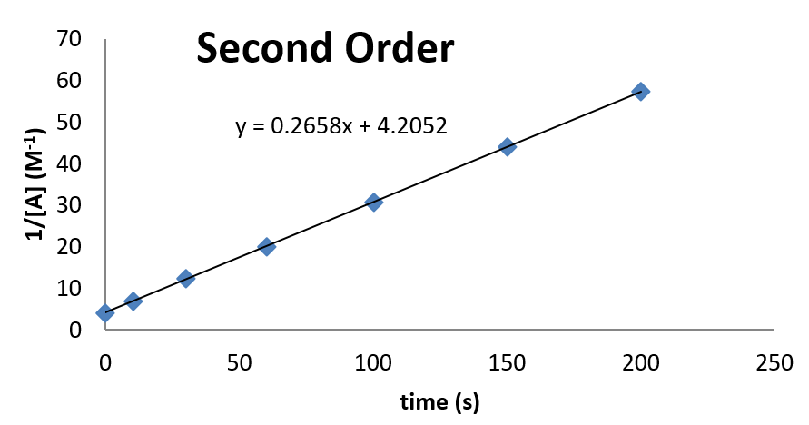
From this plot, it can be seen that the rate constant is 0.2658 M-1 s-1. The concentration at time \(t = 0\) can also be inferred from the intercept.
[1] This integral form can be generated by using the method of partial fractions. See (House, 2007) for a full derivation.
Dinitrogen pentoxide (N2O5) decomposes to NO2 and O2 at relatively low temperatures in the following reaction:
\( 2N_{2}O_{5}\left ( soln \right ) \rightarrow 4NO_{2}\left ( soln \right )+O_{2}\left ( g \right ) \)
This reaction is carried out in a CCl4 solution at 45°C. The concentrations of N2O5 as a function of time are listed in the following table, together with the natural logarithms and reciprocal N2O5 concentrations. Plot a graph of the concentration versus t, ln concentration versus t, and 1/concentration versus t and then determine the rate law and calculate the rate constant.
| Time (s) | [N2O5] (M) | ln[N2O5] | 1/[N2O5] (M−1) |
|---|---|---|---|
| 0 | 0.0365 | −3.310 | 27.4 |
| 600 | 0.0274 | −3.597 | 36.5 |
| 1200 | 0.0206 | −3.882 | 48.5 |
| 1800 | 0.0157 | −4.154 | 63.7 |
| 2400 | 0.0117 | −4.448 | 85.5 |
| 3000 | 0.00860 | −4.756 | 116 |
| 3600 | 0.00640 | −5.051 | 156 |
Given: balanced chemical equation, reaction times, and concentrations
Asked for: graph of data, rate law, and rate constant
Strategy:
A Use the data in the table to separately plot concentration, the natural logarithm of the concentration, and the reciprocal of the concentration (the vertical axis) versus time (the horizontal axis). Compare the graphs with those in Figure 13.4.2 to determine the reaction order.
B Write the rate law for the reaction. Using the appropriate data from the table and the linear graph corresponding to the rate law for the reaction, calculate the slope of the plotted line to obtain the rate constant for the reaction.
Solution:
A Here are plots of [N2O5] versus t, ln[N2O5] versus t, and 1/[N2O5] versus t:
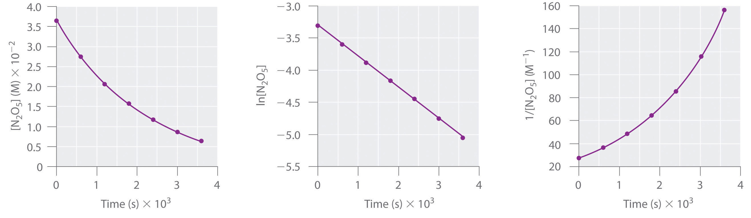
The plot of ln[N2O5] versus t gives a straight line, whereas the plots of [N2O5] versus t and 1/[N2O5] versus t do not. This means that the decomposition of N2O5 is first order in [N2O5].
B The rate law for the reaction is therefore
\( rate = k \left [N_{2}O_{5} \right ]\)
Calculating the rate constant is straightforward because we know that the slope of the plot of ln[A] versus t for a first-order reaction is −k. We can calculate the slope using any two points that lie on the line in the plot of ln[N2O5] versus t. Using the points for t = 0 and 3000 s,
\( slope= \dfrac{ln\left [N_{2}O_{5} \right ]_{3000}-ln\left [N_{2}O_{5} \right ]_{0}}{3000\;s-0\;s} = \dfrac{\left [-4.756 \right ]-\left [-3.310 \right ]}{3000\;s} =4.820\times 10^{-4}\;s^{-1} \)
Thus k = 4.820 × 10⁻⁴ s−1.
Contributors
- Anonymous
Modified by Joshua Halpern (Howard University), Scott Sinex, and Scott Johnson (PGCC)