23.2: Gibbs Energies and Phase Diagrams

First Order Transitions

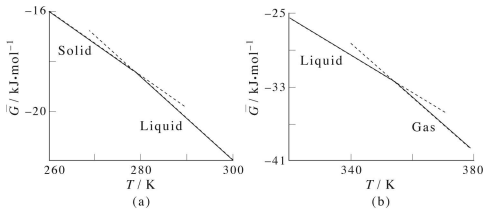
The following plot shows the Gibbs energy as a function of temperature, including phase changes from solid to liquid (melting) and liquid to gas (boiling).

Gibbs energy (\(\bar{G}\)) as a function of temperature (\(T\)).

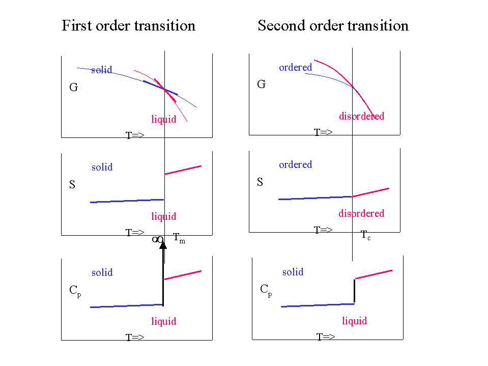
Although the \(G\) curve is continuous, its first order derivatives (\(-S\)) is discontinuous at the phase changes. This is why this transition it called a first order transition. We could say that:

• \(G\) is continuous but has a kink
• The first order derivatives (\(H\),\(S\),..) are discontinuous (have a jump)
• The second order derivatives (\(C_P\), ..) have a singularity (go to ∞)

Second Order Transitions

More subtle transitions where \(G\) is continuous, \(H\) and \(S\) are also continuous but have a kink and the discontinuity is only found in the second order derivatives (such as \(C_P\)) also exist. They are called second order transitions. In such a case:

• \(G\) is continuous and has no kink
• The first order derivatives (\(H\),\(S\),..) are continuous (but have a kink)
• The second order derivatives (\(C_P\), ..) are discontinuous (have a jump)

Table 23.2.1: Properties of Phase Transitions

Transition Order	Function	1^st Order	2^nd Order
0	G,A	kink	smooth
1	H,S,V,..	jump	kink
2	CP,CV,α,κ	sing. ∞	jump

This classification goes back to Ehrenfest. Obviously it based on the question: what order derivative is the first to go discontinuous? Of course we could extend this principle and define third order transitions but there are reasons to be doubtful that such things exist. Another problem is that it is assumed that the order must be integer: 1,2, etc. Is it possible to have a transition of intermediate non-integer order, say 1.3? Although derivatives of fractional order are beyond the scope of the chemistry curriculum the mathematics does exist (Liouville).

Schematic comparison of \(G\), \(S\) and \(C_P\) for 1st and 2nd order transitions

The Gibbs free energy is a particularly important function in the study of phases and phase transitions. The behavior of \(G(N, P,T)\), particularly as a function of \(P\) and \(T\), can signify a phase transition and can tell us some of the thermodynamic properties of different phases.

Figure 13.4: Some of the ice polymorphs.

Consider, first, the behavior of \(G\) vs. \(T\) between the solid and liquid phases of benzene: We immediately notice several things. First, although the free energy is continuous across the phase transition, its first derivative, \(\partial G/\partial T\) is not: The slope of \(G(T)\) in the solid region is different from the slope in the liquid region. When the first derivative of the free energy with respect to one of its dependent thermodynamic variables is discontinuous across a phase transition, this is an example of what is called a first order phase transition. The solid-liquid-gas phase transition of most substances is first order. When the free energy exhibits continuous first derivatives but discontinuous second derivatives, the phase transition is called second order. Examples of this type of phase transition are the order-disorder transition in paramagnetic materials.

Figure 13.5: Behavior of the Gibbs free energy across the solid-liquid phase (left) and liquid-gas (right) transitions for benzene.

Now, recall that

\[S = -\dfrac{\partial G}{\partial T} \label{13.1}\]

Consider the slopes in the solid and liquid parts of the graph:

\[\dfrac{\partial G^\text{(solid)}}{\partial T} = -S^\text{(solid)}, \: \: \: \: \: \: \: \dfrac{\partial G^\text{(liquid)}}{\partial T} = -S^\text{(liquid)} \label{13.2}\]

However, since

\[\dfrac{\partial G^\text{(liquid)}}{\partial T} < \dfrac{\partial G^\text{(solid)}}{\partial T} \label{13.3}\]

(note that the slopes are all negative, and the slope of the liquid line is more negative than that of the solid line), it follows that \(-S^\text{(liquid)} < -S^\text{(solid)}\) or \(S^\text{(liquid)} > S^\text{(solid)}\). This is what we might expect considering that the liquid phase is higher in entropy than the solid phase. The same argument can be made with regards to the gaseous phase.

Similarly, if we consider the dependence of \(G\) on pressure, we obtain a curve like that shown in the figure below:

Figure 13.6: Dependence of the Gibbs free energy as a function of pressure for benzene (left) and water (right). For benzene, the temperature is above the triple point, whereas for water, it is set below triple point.

As noted previously, here again, we see that the first derivative of \(\bar{G} (P)\) is discontinuous, signifying a first-order phase transition. Recalling that the average molar volume is

\[\bar{V} = \dfrac{\partial \bar{G}}{\partial P} \label{13.4}\]

From the graph, we see that the slopes obey

\[\bar{V}^\text{(gas)} \gg \bar{V}^\text{(liquid)} > \bar{V}^\text{(solid)} \label{13.5}\]

as one might expect for a normal substance like benzene at a temperature above its triple point. Because the temperature is above the triple point, the free energy follows a continuous path (even though it is not everywhere differentiable) from gas to liquid to solid.

On the other hand, for water, we see something a bit different, namely, that

\[\bar{V}^\text{(gas)} \gg \bar{V}^\text{(solid)} > \bar{V}^\text{(liquid)} \label{13.6}\]

at a temperature below the triple point. This, again, indicates, the unusual property of water that its solid phase is less dense than its liquid phase in the coexistence region.

Interestingly, if we look at how the plot of \(G(P)\) changes with \(T\), we obtain a plot like that shown below: Below the triple point, it is easy to see from the benzene phase diagram that the system proceeds directly from solid to gas. There is a liquid curve on this plot that is completely disconnected from the gas-solid curve, suggesting that, below the triple point, the liquid state can exist metastably if at all. AT the triple point, the solid can transition into the liquid or gas phases depending on the value of the free energy. Near the critical temperature, we see the liquid-gas transition line, while the solid line is disconnected. Above the critical temperature, the system exists as a supercritical fluid, which is shown on the lower line, and this line now shows derivative discontinuity.

Figure 13.7: Behavior of the Gibbs free energy as a function of \(P\) across different phases at different temperatures for benzene. (a): Temperature is less than the triple point; (b): Temperature is equal to the triple point; (c): Temperature is just below the critical temperature; (d): Temperature is greater than the critical temperature.

Conjugate Variables

As discussed before there are many other forms of work possible, such as electrical work, magnetic work or elastic work. These they are commonly incorporated in the formalism of thermodynamics by adding other terms, e.g:

\[dG = -SdT + VdP + ℰde + MdH + FdL + γdA \nonumber \]

1. ℰde stands for the electromotoric force ℰ and de the amount of charge transported against it.
2. MdH stand for magnetization and (change in) magnetic field.
3. F stands for the elastic force of e.g. a rubber band dL for the length it is stretched
4. γ stands for the surface tension (e.g. of a soap bubble), A for its surafce area.

The terms always appear in a pair of what is known as conjugate variables. That is even clearer if we write out the state function rather than its differential form:

\[G = U + PV -TS + ℰe + MH + FL + γA + ... \nonumber \]

The PV term can also be generalized -and needs to be so- for a viscous fluid to a stress-strain conjugate pair. It then involves a stress tensor. We will soon encounter another conjugate pair: μdn that deals with changes in composition (n) and the thermodynamic potential μ.