8.5: The Clausius-Clapeyron Equation
- Page ID
- 84340
\( \newcommand{\vecs}[1]{\overset { \scriptstyle \rightharpoonup} {\mathbf{#1}} } \)
\( \newcommand{\vecd}[1]{\overset{-\!-\!\rightharpoonup}{\vphantom{a}\smash {#1}}} \)
\( \newcommand{\id}{\mathrm{id}}\) \( \newcommand{\Span}{\mathrm{span}}\)
( \newcommand{\kernel}{\mathrm{null}\,}\) \( \newcommand{\range}{\mathrm{range}\,}\)
\( \newcommand{\RealPart}{\mathrm{Re}}\) \( \newcommand{\ImaginaryPart}{\mathrm{Im}}\)
\( \newcommand{\Argument}{\mathrm{Arg}}\) \( \newcommand{\norm}[1]{\| #1 \|}\)
\( \newcommand{\inner}[2]{\langle #1, #2 \rangle}\)
\( \newcommand{\Span}{\mathrm{span}}\)
\( \newcommand{\id}{\mathrm{id}}\)
\( \newcommand{\Span}{\mathrm{span}}\)
\( \newcommand{\kernel}{\mathrm{null}\,}\)
\( \newcommand{\range}{\mathrm{range}\,}\)
\( \newcommand{\RealPart}{\mathrm{Re}}\)
\( \newcommand{\ImaginaryPart}{\mathrm{Im}}\)
\( \newcommand{\Argument}{\mathrm{Arg}}\)
\( \newcommand{\norm}[1]{\| #1 \|}\)
\( \newcommand{\inner}[2]{\langle #1, #2 \rangle}\)
\( \newcommand{\Span}{\mathrm{span}}\) \( \newcommand{\AA}{\unicode[.8,0]{x212B}}\)
\( \newcommand{\vectorA}[1]{\vec{#1}} % arrow\)
\( \newcommand{\vectorAt}[1]{\vec{\text{#1}}} % arrow\)
\( \newcommand{\vectorB}[1]{\overset { \scriptstyle \rightharpoonup} {\mathbf{#1}} } \)
\( \newcommand{\vectorC}[1]{\textbf{#1}} \)
\( \newcommand{\vectorD}[1]{\overrightarrow{#1}} \)
\( \newcommand{\vectorDt}[1]{\overrightarrow{\text{#1}}} \)
\( \newcommand{\vectE}[1]{\overset{-\!-\!\rightharpoonup}{\vphantom{a}\smash{\mathbf {#1}}}} \)
\( \newcommand{\vecs}[1]{\overset { \scriptstyle \rightharpoonup} {\mathbf{#1}} } \)
\( \newcommand{\vecd}[1]{\overset{-\!-\!\rightharpoonup}{\vphantom{a}\smash {#1}}} \)
\(\newcommand{\avec}{\mathbf a}\) \(\newcommand{\bvec}{\mathbf b}\) \(\newcommand{\cvec}{\mathbf c}\) \(\newcommand{\dvec}{\mathbf d}\) \(\newcommand{\dtil}{\widetilde{\mathbf d}}\) \(\newcommand{\evec}{\mathbf e}\) \(\newcommand{\fvec}{\mathbf f}\) \(\newcommand{\nvec}{\mathbf n}\) \(\newcommand{\pvec}{\mathbf p}\) \(\newcommand{\qvec}{\mathbf q}\) \(\newcommand{\svec}{\mathbf s}\) \(\newcommand{\tvec}{\mathbf t}\) \(\newcommand{\uvec}{\mathbf u}\) \(\newcommand{\vvec}{\mathbf v}\) \(\newcommand{\wvec}{\mathbf w}\) \(\newcommand{\xvec}{\mathbf x}\) \(\newcommand{\yvec}{\mathbf y}\) \(\newcommand{\zvec}{\mathbf z}\) \(\newcommand{\rvec}{\mathbf r}\) \(\newcommand{\mvec}{\mathbf m}\) \(\newcommand{\zerovec}{\mathbf 0}\) \(\newcommand{\onevec}{\mathbf 1}\) \(\newcommand{\real}{\mathbb R}\) \(\newcommand{\twovec}[2]{\left[\begin{array}{r}#1 \\ #2 \end{array}\right]}\) \(\newcommand{\ctwovec}[2]{\left[\begin{array}{c}#1 \\ #2 \end{array}\right]}\) \(\newcommand{\threevec}[3]{\left[\begin{array}{r}#1 \\ #2 \\ #3 \end{array}\right]}\) \(\newcommand{\cthreevec}[3]{\left[\begin{array}{c}#1 \\ #2 \\ #3 \end{array}\right]}\) \(\newcommand{\fourvec}[4]{\left[\begin{array}{r}#1 \\ #2 \\ #3 \\ #4 \end{array}\right]}\) \(\newcommand{\cfourvec}[4]{\left[\begin{array}{c}#1 \\ #2 \\ #3 \\ #4 \end{array}\right]}\) \(\newcommand{\fivevec}[5]{\left[\begin{array}{r}#1 \\ #2 \\ #3 \\ #4 \\ #5 \\ \end{array}\right]}\) \(\newcommand{\cfivevec}[5]{\left[\begin{array}{c}#1 \\ #2 \\ #3 \\ #4 \\ #5 \\ \end{array}\right]}\) \(\newcommand{\mattwo}[4]{\left[\begin{array}{rr}#1 \amp #2 \\ #3 \amp #4 \\ \end{array}\right]}\) \(\newcommand{\laspan}[1]{\text{Span}\{#1\}}\) \(\newcommand{\bcal}{\cal B}\) \(\newcommand{\ccal}{\cal C}\) \(\newcommand{\scal}{\cal S}\) \(\newcommand{\wcal}{\cal W}\) \(\newcommand{\ecal}{\cal E}\) \(\newcommand{\coords}[2]{\left\{#1\right\}_{#2}}\) \(\newcommand{\gray}[1]{\color{gray}{#1}}\) \(\newcommand{\lgray}[1]{\color{lightgray}{#1}}\) \(\newcommand{\rank}{\operatorname{rank}}\) \(\newcommand{\row}{\text{Row}}\) \(\newcommand{\col}{\text{Col}}\) \(\renewcommand{\row}{\text{Row}}\) \(\newcommand{\nul}{\text{Nul}}\) \(\newcommand{\var}{\text{Var}}\) \(\newcommand{\corr}{\text{corr}}\) \(\newcommand{\len}[1]{\left|#1\right|}\) \(\newcommand{\bbar}{\overline{\bvec}}\) \(\newcommand{\bhat}{\widehat{\bvec}}\) \(\newcommand{\bperp}{\bvec^\perp}\) \(\newcommand{\xhat}{\widehat{\xvec}}\) \(\newcommand{\vhat}{\widehat{\vvec}}\) \(\newcommand{\uhat}{\widehat{\uvec}}\) \(\newcommand{\what}{\widehat{\wvec}}\) \(\newcommand{\Sighat}{\widehat{\Sigma}}\) \(\newcommand{\lt}{<}\) \(\newcommand{\gt}{>}\) \(\newcommand{\amp}{&}\) \(\definecolor{fillinmathshade}{gray}{0.9}\)The Clapeyron equation can be developed further for phase equilibria involving the gas phase as one of the phases. This is the case for either sublimation (\(\text{solid} \rightarrow \text{gas}\)) or vaporization (\(\text{liquid} \rightarrow \text{gas}\)). In the case of vaporization, the change in molar volume can be expressed
\[ \Delta V = V_{gas} -V_{liquid} \nonumber \]
Since substances undergo a very large increase in molar volume upon vaporization, the molar volume of the condensed phase (liquid in this case) is negligibly small compared to the molar volume of the gas (i.e., \(V_{gas} \gg V_{liquid}\)). So,
\[\Delta V \approx V_{gas} \nonumber \]
And if the vapor can be treated as an ideal gas,
\[V_{gas} = \dfrac{RT}{p} \nonumber \]
Substitution into the Claperyron equation yields
\[\dfrac{dp}{dT} = \dfrac{p\Delta H_{vap}}{RT^2} \nonumber \]
Separating the variables puts the equation into an integrable form.
\[dp = \dfrac{p\Delta H_{vap}}{R} \dfrac{dT}{T^2} \label{diffCC} \]
Noting that
\[\dfrac{dT}{T^2} =- d\left(\dfrac{1}{T} \right) \nonumber \]
makes the integration very easy. If the enthalpy of vaporization is independent of temperature over the range of conditions,
\[ \int_{p_1}^{p_2} \dfrac{dp}{p} = - \dfrac{\Delta H_{vap}}{R} \int_{T_1}^{T_2} d\left(\dfrac{1}{T} \right) \nonumber \]
\[ \ln \left( \dfrac{p_2}{p_1}\right) = - \dfrac{\Delta H_{vap}}{R} \left( \dfrac{1}{T_2} -\dfrac{1}{T_1} \right) \label{CC} \]
This is the Clausius-Clapeyron equation. It can also be used to describe the boundary between solid and vapor phases by substituting the enthalpy of sublimation (\(\Delta H_{sub}\))
The vapor pressure of a liquid triples when the temperature is increased from 25 °C to 45 °C. What is the enthalpy of vaporization for the liquid?
Solution
The problem can be solved using the Clausius-Clapeyron equation (Equation \ref{CC}). The following values can be used:
| \(p_2 = 3 p_1\) | \(T_2 = 318\, K\) |
| \(p_1 = p_1\) | \(T_1 = 298\, K\) |
Substitution into the Clausius-Clapeyron equation yields
\[ \ln \left( \dfrac{3p_1}{p_1}\right) = - \dfrac{\Delta H_{vap}}{9.314 \dfrac{J}{mol\,K}} \left( \dfrac{1}{318\,K} -\dfrac{1}{298\,K} \right) \nonumber \]
\[ \Delta H_{vap} = 43280 \,\dfrac{J}{mol} = 43.28 \, \dfrac{kJ}{mol} \nonumber \]
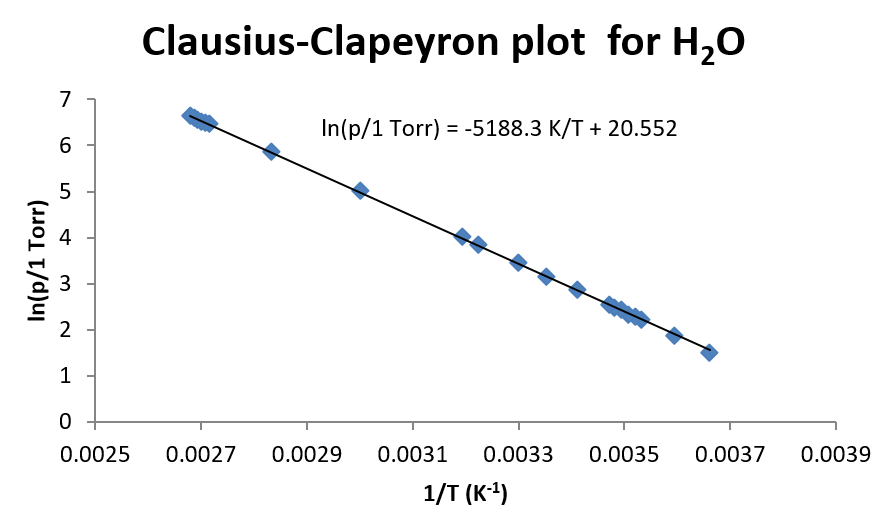
The Clausius-Clapeyron equation also suggests that a plot of \(\ln(p)\) vs. \(1/T\) should yield a straight line, the slope of which is \(–\Delta H/R\) (provided that \(\Delta H_{vap}\) is independent of temperature over the range of temperatures involved..
\[ \ln(p) = - \dfrac{\Delta H_{vap}}{R} \left( \dfrac{1}{T} \right) + const. \nonumber \]
This approach in Example \(\PageIndex{1}\) is very useful when there are several pairs of measurements of vapor pressure and temperature. Such a plot is shown below for water.

For water, which has a very large temperature dependence, the linear relationship of \(\ln(p)\) vs. \(1/T\) holds fairly well over a broad range of temperatures. So even though there is some curvature to the data, a straight line fit still results in a reasonable description of the data (depending, of course, on the precision needed in the experiment.) For this fit of the data, \(\Delta H_{vap}\) is found to be 43.14 kJ/mol.
Temperature Dependence to \(\Delta H_{vap}\)
For systems that warrant it, temperature dependence of \(\Delta H_{vap}\) can be included into the derivation of the model to fit vapor pressure as a function of temperature. For example, if the enthalpy of vaporization is assumed to take the following empirical form
\[ \Delta H_{vap} = \Delta H_o + aT + bT^2 \nonumber \]
and substituting it into the differential form of the Clausius-Clapeyron equation (Equation \ref{diffCC}) generates
\[ \dfrac{dp}{p} = \dfrac{\Delta H_o + aT + bT^2}{R} \dfrac{dT}{T^2} \nonumber \]
or
\[ \dfrac{dp}{p} = \dfrac{\Delta H_o}{R} \dfrac{dT}{T^2} + \dfrac{a}{R} \dfrac{dT}{T} + \dfrac{b}{R} dT \nonumber \]
And so the integrated form becomes
\[ \ln (p) = - \dfrac{\Delta H_o}{R} \left(\dfrac{1}{T}\right) + \dfrac{a}{R} \ln T + \dfrac{b}{R} T + constant \nonumber \]
The results of fitting these data to the temperature dependent model are shown in the table below.
| \(\Delta H_0\) (J mol-1) | a (J mol-1 K-1) | b (J mol-1 K-2) | c |
|---|---|---|---|
| 43080 | 0.01058 | 0.000501 | 20.50 |
This results in calculated values of \(\Delta H_{vap}\) of 43.13 kJ/mol at 298 K, and 43.15 kJ/mol at 373 K. The results are a little bit skewed since there is no data above 100 oC included in the fit. A larger temperature dependence would be found if the higher-temperature data were included in the fit.


