4.5: The Joule-Thomson Effect
- Page ID
- 84312
\( \newcommand{\vecs}[1]{\overset { \scriptstyle \rightharpoonup} {\mathbf{#1}} } \)
\( \newcommand{\vecd}[1]{\overset{-\!-\!\rightharpoonup}{\vphantom{a}\smash {#1}}} \)
\( \newcommand{\id}{\mathrm{id}}\) \( \newcommand{\Span}{\mathrm{span}}\)
( \newcommand{\kernel}{\mathrm{null}\,}\) \( \newcommand{\range}{\mathrm{range}\,}\)
\( \newcommand{\RealPart}{\mathrm{Re}}\) \( \newcommand{\ImaginaryPart}{\mathrm{Im}}\)
\( \newcommand{\Argument}{\mathrm{Arg}}\) \( \newcommand{\norm}[1]{\| #1 \|}\)
\( \newcommand{\inner}[2]{\langle #1, #2 \rangle}\)
\( \newcommand{\Span}{\mathrm{span}}\)
\( \newcommand{\id}{\mathrm{id}}\)
\( \newcommand{\Span}{\mathrm{span}}\)
\( \newcommand{\kernel}{\mathrm{null}\,}\)
\( \newcommand{\range}{\mathrm{range}\,}\)
\( \newcommand{\RealPart}{\mathrm{Re}}\)
\( \newcommand{\ImaginaryPart}{\mathrm{Im}}\)
\( \newcommand{\Argument}{\mathrm{Arg}}\)
\( \newcommand{\norm}[1]{\| #1 \|}\)
\( \newcommand{\inner}[2]{\langle #1, #2 \rangle}\)
\( \newcommand{\Span}{\mathrm{span}}\) \( \newcommand{\AA}{\unicode[.8,0]{x212B}}\)
\( \newcommand{\vectorA}[1]{\vec{#1}} % arrow\)
\( \newcommand{\vectorAt}[1]{\vec{\text{#1}}} % arrow\)
\( \newcommand{\vectorB}[1]{\overset { \scriptstyle \rightharpoonup} {\mathbf{#1}} } \)
\( \newcommand{\vectorC}[1]{\textbf{#1}} \)
\( \newcommand{\vectorD}[1]{\overrightarrow{#1}} \)
\( \newcommand{\vectorDt}[1]{\overrightarrow{\text{#1}}} \)
\( \newcommand{\vectE}[1]{\overset{-\!-\!\rightharpoonup}{\vphantom{a}\smash{\mathbf {#1}}}} \)
\( \newcommand{\vecs}[1]{\overset { \scriptstyle \rightharpoonup} {\mathbf{#1}} } \)
\( \newcommand{\vecd}[1]{\overset{-\!-\!\rightharpoonup}{\vphantom{a}\smash {#1}}} \)
\(\newcommand{\avec}{\mathbf a}\) \(\newcommand{\bvec}{\mathbf b}\) \(\newcommand{\cvec}{\mathbf c}\) \(\newcommand{\dvec}{\mathbf d}\) \(\newcommand{\dtil}{\widetilde{\mathbf d}}\) \(\newcommand{\evec}{\mathbf e}\) \(\newcommand{\fvec}{\mathbf f}\) \(\newcommand{\nvec}{\mathbf n}\) \(\newcommand{\pvec}{\mathbf p}\) \(\newcommand{\qvec}{\mathbf q}\) \(\newcommand{\svec}{\mathbf s}\) \(\newcommand{\tvec}{\mathbf t}\) \(\newcommand{\uvec}{\mathbf u}\) \(\newcommand{\vvec}{\mathbf v}\) \(\newcommand{\wvec}{\mathbf w}\) \(\newcommand{\xvec}{\mathbf x}\) \(\newcommand{\yvec}{\mathbf y}\) \(\newcommand{\zvec}{\mathbf z}\) \(\newcommand{\rvec}{\mathbf r}\) \(\newcommand{\mvec}{\mathbf m}\) \(\newcommand{\zerovec}{\mathbf 0}\) \(\newcommand{\onevec}{\mathbf 1}\) \(\newcommand{\real}{\mathbb R}\) \(\newcommand{\twovec}[2]{\left[\begin{array}{r}#1 \\ #2 \end{array}\right]}\) \(\newcommand{\ctwovec}[2]{\left[\begin{array}{c}#1 \\ #2 \end{array}\right]}\) \(\newcommand{\threevec}[3]{\left[\begin{array}{r}#1 \\ #2 \\ #3 \end{array}\right]}\) \(\newcommand{\cthreevec}[3]{\left[\begin{array}{c}#1 \\ #2 \\ #3 \end{array}\right]}\) \(\newcommand{\fourvec}[4]{\left[\begin{array}{r}#1 \\ #2 \\ #3 \\ #4 \end{array}\right]}\) \(\newcommand{\cfourvec}[4]{\left[\begin{array}{c}#1 \\ #2 \\ #3 \\ #4 \end{array}\right]}\) \(\newcommand{\fivevec}[5]{\left[\begin{array}{r}#1 \\ #2 \\ #3 \\ #4 \\ #5 \\ \end{array}\right]}\) \(\newcommand{\cfivevec}[5]{\left[\begin{array}{c}#1 \\ #2 \\ #3 \\ #4 \\ #5 \\ \end{array}\right]}\) \(\newcommand{\mattwo}[4]{\left[\begin{array}{rr}#1 \amp #2 \\ #3 \amp #4 \\ \end{array}\right]}\) \(\newcommand{\laspan}[1]{\text{Span}\{#1\}}\) \(\newcommand{\bcal}{\cal B}\) \(\newcommand{\ccal}{\cal C}\) \(\newcommand{\scal}{\cal S}\) \(\newcommand{\wcal}{\cal W}\) \(\newcommand{\ecal}{\cal E}\) \(\newcommand{\coords}[2]{\left\{#1\right\}_{#2}}\) \(\newcommand{\gray}[1]{\color{gray}{#1}}\) \(\newcommand{\lgray}[1]{\color{lightgray}{#1}}\) \(\newcommand{\rank}{\operatorname{rank}}\) \(\newcommand{\row}{\text{Row}}\) \(\newcommand{\col}{\text{Col}}\) \(\renewcommand{\row}{\text{Row}}\) \(\newcommand{\nul}{\text{Nul}}\) \(\newcommand{\var}{\text{Var}}\) \(\newcommand{\corr}{\text{corr}}\) \(\newcommand{\len}[1]{\left|#1\right|}\) \(\newcommand{\bbar}{\overline{\bvec}}\) \(\newcommand{\bhat}{\widehat{\bvec}}\) \(\newcommand{\bperp}{\bvec^\perp}\) \(\newcommand{\xhat}{\widehat{\xvec}}\) \(\newcommand{\vhat}{\widehat{\vvec}}\) \(\newcommand{\uhat}{\widehat{\uvec}}\) \(\newcommand{\what}{\widehat{\wvec}}\) \(\newcommand{\Sighat}{\widehat{\Sigma}}\) \(\newcommand{\lt}{<}\) \(\newcommand{\gt}{>}\) \(\newcommand{\amp}{&}\) \(\definecolor{fillinmathshade}{gray}{0.9}\)In 1852, working with William Thomson (who would later become Lord Kelvin), Joule conducted an experiment in which they pumped gas at a steady rate through a lead pipe that was cinched to create a construction. On the upstream side of the constriction, the gas was at a higher pressure than on the downstream side of the constriction. Also, the temperature of the gas was carefully monitored on either side of the construction. The cooling that they observed as the gas expanded from a high pressure region to a lower pressure region was extremely important and lead to a common design of modern refrigerators.
Not all gases undergo a cooling effect upon expansion. Some gases, such as hydrogen and helium, will experience a warming effect upon expansion under conditions near room temperature and pressure. The direction of temperature change can be determined by measuring the Joule-Thomson coefficient, \(\mu_{JT}\). This coefficient has the definition
\[ \mu_{JT} \equiv \left( \dfrac{\partial T}{\partial p} \right)_H \nonumber \]
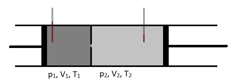
Schematically, the Joule-Thomson coefficient can be measured by measuring the temperature drop or increase a gas undergoes for a given pressure drop (Figure \(\PageIndex{1}\)). The apparatus is insulated so that no heat can be transferred in or out, making the expansion isenthalpic.

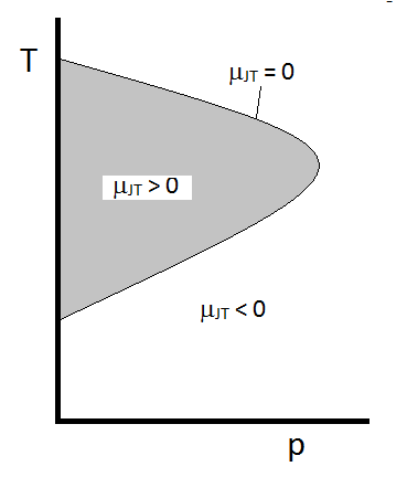
The typical behavior of the Joule-Thomson coefficient can be summarized in Figure \(\PageIndex{2}\). At the combinations of \(T\) and \(p\) for which \(\mu_{JT} > 0\) (inside the shaded region), the sample will cool upon expansion. At those \(p\) and \(T\) conditions outside of the shaded region, where \(\mu_{JT} < 0\), the gas will undergo a temperature increase upon expansion. And along the boundary, a gas will undergo neither a temperature increase not decrease upon expansion. For a given pressure, there are typically two temperatures at which \(\mu_{JT}\) changes sign. These are the upper and lower inversion temperatures.

Using the tools of mathematics, it is possible to express the Joule-Thomson coefficient in terms of measurable properties. Consider enthalpy as a function of pressure and temperature: \(H(p, T)\). This suggests that the total differential \(dH\) can be expressed
\[dH= \left( \dfrac{\partial H}{\partial p} \right)_T dp+ \left( \dfrac{\partial H}{\partial T} \right)_p dT \label{totalH} \]
It will be shown later (again, once we develop the Maxwell Relations) that
\[\left( \dfrac{\partial H}{\partial p} \right)_T dp = -T \left( \dfrac{\partial V}{\partial T} \right)_p + V \nonumber \]
A simple substitution shows
\[\left( \dfrac{\partial H}{\partial p} \right)_T dp = - TV \alpha + V = V(1-T\alpha) \nonumber \]
So
\[ dH = V(1-T\alpha) dP + C_p dT \nonumber \]
For an ideal gas, \(\alpha = 1/T\), so
\[ dH = \cancelto{0}{V\left(1-T\dfrac{1}{T}\right) dP} + C_p dT \nonumber \]
which causes the first term to vanish. So for constant enthalpy expansion (\(dH = 0\)), there can be no change in temperature (\(dT = 0\)). This will mean that gases will only show non-zero values for \(\mu_{JT}\) only because they deviate from ideal behavior!
Derive an expression for \(\mu_{JT}\) in terms of \(\alpha\), \(C_p\), \(V\), and \(T\).
Solution
Using the total differential for \(H(p, T)\) (Equation \ref{totalH}):
\[dH= \left( \dfrac{\partial H}{\partial p} \right)_T dp+ \left( \dfrac{\partial H}{\partial T} \right)_p dT \nonumber \]
Dividing by \(dp\) and constraining to constant \(H\):
\[\left.\dfrac{dH}{dp} \right\rvert_{H}= \left( \dfrac{\partial H}{\partial p} \right)_T \left.\dfrac{dp}{dp} \right\rvert_{H} + \left( \dfrac{\partial H}{\partial T} \right)_p \left.\dfrac{dT}{dp} \right\rvert_{H} \nonumber \]
Noting that
\[\left.\dfrac{dH}{dp} \right\rvert_{H} = 0 \nonumber \]
\[\left.\dfrac{dp}{dp} \right\rvert_{H} = 1 \nonumber \]
and
\[\left.\dfrac{dT}{dp} \right\rvert_{H} = \left(\dfrac{\partial T}{\partial p} \right)_{H} \nonumber \]
so
\[ 0 = \left( \dfrac{\partial H}{\partial p} \right)_T + \left( \dfrac{\partial H}{\partial T} \right)_p \left(\dfrac{\partial T}{\partial p} \right)_{H} \nonumber \]
We can then use the following substitutions:
\[\left( \dfrac{\partial H}{\partial p} \right)_T = V(1-T \alpha) \nonumber \]
\[\left( \dfrac{\partial H}{\partial T} \right)_p = C_p \nonumber \]
\[\left(\dfrac{\partial T}{\partial p} \right)_{H} = \mu_{JT} \nonumber \]
To get
\[ 0 = V(1-T \alpha) + C_p \mu_{JT} \nonumber \]
And solving for \(\mu_{JT}\) gives
\[\mu_{JT} = \dfrac{V}{C_p}(T \alpha -1) \nonumber \]


