
1.4: The Hydrogen Atomic Spectrum
- Page ID
- 13384
\( \newcommand{\vecs}[1]{\overset { \scriptstyle \rightharpoonup} {\mathbf{#1}} } \)
\( \newcommand{\vecd}[1]{\overset{-\!-\!\rightharpoonup}{\vphantom{a}\smash {#1}}} \)
\( \newcommand{\id}{\mathrm{id}}\) \( \newcommand{\Span}{\mathrm{span}}\)
( \newcommand{\kernel}{\mathrm{null}\,}\) \( \newcommand{\range}{\mathrm{range}\,}\)
\( \newcommand{\RealPart}{\mathrm{Re}}\) \( \newcommand{\ImaginaryPart}{\mathrm{Im}}\)
\( \newcommand{\Argument}{\mathrm{Arg}}\) \( \newcommand{\norm}[1]{\| #1 \|}\)
\( \newcommand{\inner}[2]{\langle #1, #2 \rangle}\)
\( \newcommand{\Span}{\mathrm{span}}\)
\( \newcommand{\id}{\mathrm{id}}\)
\( \newcommand{\Span}{\mathrm{span}}\)
\( \newcommand{\kernel}{\mathrm{null}\,}\)
\( \newcommand{\range}{\mathrm{range}\,}\)
\( \newcommand{\RealPart}{\mathrm{Re}}\)
\( \newcommand{\ImaginaryPart}{\mathrm{Im}}\)
\( \newcommand{\Argument}{\mathrm{Arg}}\)
\( \newcommand{\norm}[1]{\| #1 \|}\)
\( \newcommand{\inner}[2]{\langle #1, #2 \rangle}\)
\( \newcommand{\Span}{\mathrm{span}}\) \( \newcommand{\AA}{\unicode[.8,0]{x212B}}\)
\( \newcommand{\vectorA}[1]{\vec{#1}} % arrow\)
\( \newcommand{\vectorAt}[1]{\vec{\text{#1}}} % arrow\)
\( \newcommand{\vectorB}[1]{\overset { \scriptstyle \rightharpoonup} {\mathbf{#1}} } \)
\( \newcommand{\vectorC}[1]{\textbf{#1}} \)
\( \newcommand{\vectorD}[1]{\overrightarrow{#1}} \)
\( \newcommand{\vectorDt}[1]{\overrightarrow{\text{#1}}} \)
\( \newcommand{\vectE}[1]{\overset{-\!-\!\rightharpoonup}{\vphantom{a}\smash{\mathbf {#1}}}} \)
\( \newcommand{\vecs}[1]{\overset { \scriptstyle \rightharpoonup} {\mathbf{#1}} } \)
\( \newcommand{\vecd}[1]{\overset{-\!-\!\rightharpoonup}{\vphantom{a}\smash {#1}}} \)
\(\newcommand{\avec}{\mathbf a}\) \(\newcommand{\bvec}{\mathbf b}\) \(\newcommand{\cvec}{\mathbf c}\) \(\newcommand{\dvec}{\mathbf d}\) \(\newcommand{\dtil}{\widetilde{\mathbf d}}\) \(\newcommand{\evec}{\mathbf e}\) \(\newcommand{\fvec}{\mathbf f}\) \(\newcommand{\nvec}{\mathbf n}\) \(\newcommand{\pvec}{\mathbf p}\) \(\newcommand{\qvec}{\mathbf q}\) \(\newcommand{\svec}{\mathbf s}\) \(\newcommand{\tvec}{\mathbf t}\) \(\newcommand{\uvec}{\mathbf u}\) \(\newcommand{\vvec}{\mathbf v}\) \(\newcommand{\wvec}{\mathbf w}\) \(\newcommand{\xvec}{\mathbf x}\) \(\newcommand{\yvec}{\mathbf y}\) \(\newcommand{\zvec}{\mathbf z}\) \(\newcommand{\rvec}{\mathbf r}\) \(\newcommand{\mvec}{\mathbf m}\) \(\newcommand{\zerovec}{\mathbf 0}\) \(\newcommand{\onevec}{\mathbf 1}\) \(\newcommand{\real}{\mathbb R}\) \(\newcommand{\twovec}[2]{\left[\begin{array}{r}#1 \\ #2 \end{array}\right]}\) \(\newcommand{\ctwovec}[2]{\left[\begin{array}{c}#1 \\ #2 \end{array}\right]}\) \(\newcommand{\threevec}[3]{\left[\begin{array}{r}#1 \\ #2 \\ #3 \end{array}\right]}\) \(\newcommand{\cthreevec}[3]{\left[\begin{array}{c}#1 \\ #2 \\ #3 \end{array}\right]}\) \(\newcommand{\fourvec}[4]{\left[\begin{array}{r}#1 \\ #2 \\ #3 \\ #4 \end{array}\right]}\) \(\newcommand{\cfourvec}[4]{\left[\begin{array}{c}#1 \\ #2 \\ #3 \\ #4 \end{array}\right]}\) \(\newcommand{\fivevec}[5]{\left[\begin{array}{r}#1 \\ #2 \\ #3 \\ #4 \\ #5 \\ \end{array}\right]}\) \(\newcommand{\cfivevec}[5]{\left[\begin{array}{c}#1 \\ #2 \\ #3 \\ #4 \\ #5 \\ \end{array}\right]}\) \(\newcommand{\mattwo}[4]{\left[\begin{array}{rr}#1 \amp #2 \\ #3 \amp #4 \\ \end{array}\right]}\) \(\newcommand{\laspan}[1]{\text{Span}\{#1\}}\) \(\newcommand{\bcal}{\cal B}\) \(\newcommand{\ccal}{\cal C}\) \(\newcommand{\scal}{\cal S}\) \(\newcommand{\wcal}{\cal W}\) \(\newcommand{\ecal}{\cal E}\) \(\newcommand{\coords}[2]{\left\{#1\right\}_{#2}}\) \(\newcommand{\gray}[1]{\color{gray}{#1}}\) \(\newcommand{\lgray}[1]{\color{lightgray}{#1}}\) \(\newcommand{\rank}{\operatorname{rank}}\) \(\newcommand{\row}{\text{Row}}\) \(\newcommand{\col}{\text{Col}}\) \(\renewcommand{\row}{\text{Row}}\) \(\newcommand{\nul}{\text{Nul}}\) \(\newcommand{\var}{\text{Var}}\) \(\newcommand{\corr}{\text{corr}}\) \(\newcommand{\len}[1]{\left|#1\right|}\) \(\newcommand{\bbar}{\overline{\bvec}}\) \(\newcommand{\bhat}{\widehat{\bvec}}\) \(\newcommand{\bperp}{\bvec^\perp}\) \(\newcommand{\xhat}{\widehat{\xvec}}\) \(\newcommand{\vhat}{\widehat{\vvec}}\) \(\newcommand{\uhat}{\widehat{\uvec}}\) \(\newcommand{\what}{\widehat{\wvec}}\) \(\newcommand{\Sighat}{\widehat{\Sigma}}\) \(\newcommand{\lt}{<}\) \(\newcommand{\gt}{>}\) \(\newcommand{\amp}{&}\) \(\definecolor{fillinmathshade}{gray}{0.9}\)- To introduce the concept of absorption and emission line spectra and describe the Balmer equation to describe the visible lines of atomic hydrogen.
The first person to realize that white light was made up of the colors of the rainbow was Isaac Newton, who in 1666 passed sunlight through a narrow slit, then a prism, to project the colored spectrum on to a wall. This effect had been noticed previously, of course, not least in the sky, but previous attempts to explain it, by Descartes and others, had suggested that the white light became colored when it was refracted, the color depending on the angle of refraction. Newton clarified the situation by using a second prism to reconstitute the white light, making much more plausible the idea that the white light was composed of the separate colors. He then took a monochromatic component from the spectrum generated by one prism and passed it through a second prism, establishing that no further colors were generated. That is, light of a single color did not change color on refraction. He concluded that white light was made up of all the colors of the rainbow, and that on passing through a prism, these different colors were refracted through slightly different angles, thus separating them into the observed spectrum.
Atomic Line Spectra
The spectrum of hydrogen atoms, which turned out to be crucial in providing the first insight into atomic structure over half a century later, was first observed by Anders Ångström in Uppsala, Sweden, in 1853. His communication was translated into English in 1855. Ångström, the son of a country minister, was a reserved person, not interested in the social life that centered around the court. Consequently, it was many years before his achievements were recognized, at home or abroad (most of his results were published in Swedish).


Most of what is known about atomic (and molecular) structure and mechanics has been deduced from spectroscopy. Figure 1.4.1 shows two different types of spectra. A continuous spectrum can be produced by an incandescent solid or gas at high pressure (e.g., blackbody radiation is a continuum). An emission spectrum can be produced by a gas at low pressure excited by heat or by collisions with electrons. An absorption spectrum results when light from a continuous source passes through a cooler gas, consisting of a series of dark lines characteristic of the composition of the gas.
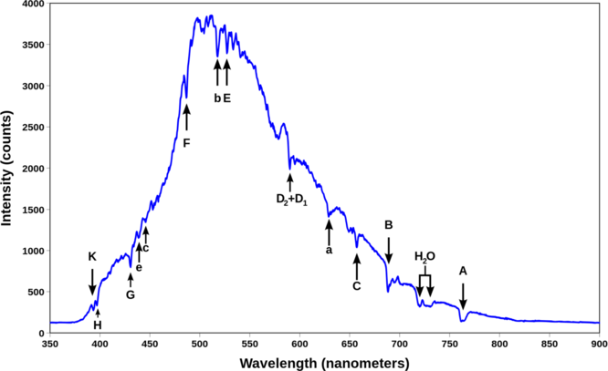
In 1802, William Wollaston in England had discovered that the solar spectrum had tiny gaps - there were many thin dark lines in the rainbow of colors. These were investigated much more systematically by Joseph von Fraunhofer, beginning in 1814. He increased the dispersion by using more than one prism. He found an "almost countless number" of lines. He labeled the strongest dark lines A, B, C, D, etc. Frauenhofer between 1814 and 1823 discovered nearly 600 dark lines in the solar spectrum viewed at high resolution and designated the principal features with the letters A through K, and weaker lines with other letters (Table 1.4.1 ). Modern observations of sunlight can detect many thousands of lines. It is now understood that these lines are caused by absorption by the outer layers of the Sun.
| Designation | Element | Wavelength (nm) |
|---|---|---|
| y | O2 | 898.765 |
| Z | O2 | 822.696 |
| A | O2 | 759.370 |
| B | O2 | 686.719 |
| C | H | 656.281 |
| a | O2 | 627.661 |
| D1 | Na | 589.592 |
| D2 | Na | 588.995 |
| D3 or d | He | 587.5618 |
The Fraunhofer lines are typical spectral absorption lines. These dark lines are produced whenever a cold gas is between a broad spectrum photon source and the detector. In this case, a decrease in the intensity of light in the frequency of the incident photon is seen as the photons are absorbed, then re-emitted in random directions, which are mostly in directions different from the original one. This results in an absorption line, since the narrow frequency band of light initially traveling toward the detector, has been turned into heat or re-emitted in other directions.
By contrast, if the detector sees photons emitted directly from a glowing gas, then the detector often sees photons emitted in a narrow frequency range by quantum emission processes in atoms in the hot gas, resulting in an emission line. In the Sun, Fraunhofer lines are seen from gas in the outer regions of the Sun, which are too cold to directly produce emission lines of the elements they represent.
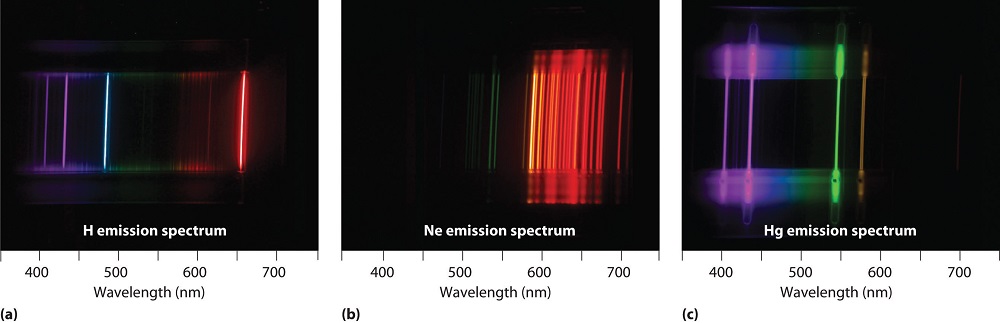
Gases heated to incandescence were found by Bunsen, Kirkhoff and others to emit light with a series of sharp wavelengths. The emitted light analyzed by a spectrometer (or even a simple prism) appears as a multitude of narrow bands of color. These so called line spectra are characteristic of the atomic composition of the gas. The line spectra of several elements are shown in Figure 1.4.3 .
The Balmer Series of Hydrogen
Obviously, if any pattern could be discerned in the spectral lines for a specific atom (in contract to the mixture that Fraunhofer lines represent), that might be a clue as to the internal structure of the atom. One might be able to build a model. A great deal of effort went into analyzing the spectral data from the 1860's on. The big breakthrough was made by Johann Balmer, a math and Latin teacher at a girls' school in Basel, Switzerland. Balmer had done no physics before and made his great discovery when he was almost sixty.
Balmer decided that the most likely atom to show simple spectral patterns was the lightest atom, hydrogen. Ångström had measured the four visible spectral lines to have wavelengths 656.21, 486.07, 434.01 and 410.12 nm (Figure 1.4.4 ). Balmer concentrated on just these four numbers, and found they were represented by the phenomenological formula:
\[\lambda = b \left( \dfrac{n_2^2}{n_2^2 -4} \right) \label{1.4.1} \]
where \(b\) = 364.56 nm and \(n_2 = 3, 4, 5, 6\).
The first four wavelengths of Equation \(\ref{1.4.1}\) (with \(n_2\) = 3, 4, 5, 6) were in excellent agreement with the experimental lines from Ångström (Table 1.4.2 ). Balmer predicted that other lines exist in the ultraviolet that correspond to \(n_2 \ge 7\) and in fact some of them had already been observed, unbeknown to Balmer.
| \(n_2\) | 3 | 4 | 5 | 6 | 7 | 8 | 9 | 10 |
|---|---|---|---|---|---|---|---|---|
| \(\lambda\) | 656 | 486 | 434 | 410 | 397 | 389 | 383 | 380 |
| color | red | teal | blue | indigo | violet | not visible | not visible | not visible |
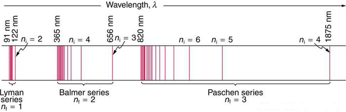
The \(n_2\) integer in the Balmer series extends theoretically to infinity and the series represents a monotonically increasing energy (and frequency) of the absorption lines with increasing \(n_2\) values. Moreover, the energy difference between successive lines decreased as \(n_2\) increases (1.4.4 ). This behavior converges to a highest possible energy as Example 1.4.1 demonstrates. If the lines are plot according to their \(\lambda\) on a linear scale, you will get the appearance of the spectrum in Figure 1.4.4 ; these lines are called the Balmer series.
Balmer's general formula (Equation \(\ref{1.4.1}\)) can be rewritten in terms of the inverse wavelength typically called the wavenumber (\(\widetilde{\nu}\)).
\[ \begin{align} \widetilde{\nu} &= \dfrac{1}{ \lambda} \\[4pt] &=R_H \left( \dfrac{1}{4} -\dfrac{1}{n_2^2}\right) \label{1.4.2} \end{align} \]
where \(n_2 = 3, 4, 5, 6\) and \(R_H\) is the Rydberg constant (discussed in the next section) equal to 109,737 cm-1.
He further conjectured that the 4 could be replaced by 9, 16, 25, … and this also turned out to be true - but these lines, further into the infrared, were not detected until the early twentieth century, along with the ultraviolet lines.
The relation between wavelength and frequency for electromagnetic radiation is
\[\lambda \nu= c \nonumber \]
In the SI system of units the wavelength, (\(\lambda\)) is measured in meters (m) and since wavelengths are usually very small one often uses the nanometer (nm) which is \(10^{-9}\; m\). The frequency (\(\nu\)) in the SI system is measured in reciprocal seconds 1/s − which is called a Hertz (after the discover of the photoelectron effect) and is represented by Hz.
It is common to use the reciprocal of the wavelength in centimeters as a measure of the frequency of radiation. This unit is called a wavenumber and is represented by (\(\widetilde{\nu}\)) and is defined by
\[ \begin{align*} \widetilde{\nu} &= \dfrac{1}{ \lambda} \\[4pt] &= \dfrac{\nu}{c} \end{align*} \nonumber \]
Wavenumbers is a convenient unit in spectroscopy because it is directly proportional to energy.
\[ \begin{align*} E &= \dfrac{hc}{\lambda} \nonumber \\[4pt] &= hc \times \dfrac{1}{\lambda} \nonumber \\[4pt] &= hc\widetilde{\nu} \label{energy} \\[4pt] &\propto \widetilde{\nu} \end{align*} \]
Calculate the longest and shortest wavelengths (in nm) emitted in the Balmer series of the hydrogen atom emission spectrum.
Solution
From the behavior of the Balmer equation (Equation \(\ref{1.4.1}\) and Table 1.4.2 ), the value of \(n_2\) that gives the longest (i.e., greatest) wavelength (\(\lambda\)) is the smallest value possible of \(n_2\), which is (\(n_2\)=3) for this series. This results in
\[ \begin{align*} \lambda_{longest} &= (364.56 \;nm) \left( \dfrac{9}{9 -4} \right) \\[4pt] &= (364.56 \;nm) \left( 1.8 \right) \\[4pt] &= 656.2\; nm \end{align*} \nonumber \]
This is also known as the \(H_{\alpha}\) line of atomic hydrogen and is bright red (Figure \(\PageIndex{3a}\)).
For the shortest wavelength, it should be recognized that the shortest wavelength (greatest energy) is obtained at the limit of greatest (\(n_2\)):
\[ \lambda_{shortest} = \lim_{n_2 \rightarrow \infty} (364.56 \;nm) \left( \dfrac{n_2^2}{n_2^2 -4} \right) \nonumber \]
This can be solved via L'Hôpital's Rule, or alternatively the limit can be expressed via the equally useful energy expression (Equation \ref{1.4.2}) and simply solved:
\[ \begin{align*} \widetilde{\nu}_{greatest} &= \lim_{n_2 \rightarrow \infty} R_H \left( \dfrac{1}{4} -\dfrac{1}{n_2^2}\right) \\[4pt] &= \lim_{n_2 \rightarrow \infty} R_H \left( \dfrac{1}{4}\right) \\[4pt] &= 27,434 \;cm^{-1} \end{align*} \nonumber \]
Since \( \dfrac{1}{\widetilde{\nu}}= \lambda\) in units of cm, this converts to 364 nm as the shortest wavelength possible for the Balmer series.
The Balmer series is particularly useful in astronomy because the Balmer lines appear in numerous stellar objects due to the abundance of hydrogen in the universe, and therefore are commonly seen and relatively strong compared to lines from other elements.
Contributors and Attributions
Michael Fowler (Beams Professor, Department of Physics, University of Virginia)