
10.1: Nitroxide spin probes and labels
- Page ID
- 370951
Spin probes and labels
Spin probes are stable paramagnetic species that are admixed to a sample in order to obtain structural or dynamical information on their environment and, thus, indirectly on the sample. Spin labels are spin probes that are covalently attached to a molecule of interest, often at a specific site. As compared to more direct characterization of structure and dynamics by other techniques, EPR spectroscopy on spin probes may be able to access other length and time scales or may be applicable in aggregation states or environments where these other techniques exhibit low resolution or do not yield any signal. Site-directed spin labeling (SDSL) has the advantage that assignment of the signal to primary molecular structure is already known and that a specific site in a complex system can be studied without disturbance from signals of other parts of the system. This approach profits from the rarity of paramagnetic centers. For instance, many proteins and most nucleic acids and lipids are diamagnetic. If a spin label is introduced at a selected site, EPR information is specific to this particular site.
In principle, any stable paramagnetic species can serve as a spin probe. Some paramagnetic metal ions can substitute for diamagnetic ions native to the system under study, as they have similar charge and ionic radius or with similar complexation properties as the native ions. This applies to \(\mathrm{Mn}(\mathrm{II})\), which can often substitute for \(\mathrm{Mg}(\mathrm{II})\) without affecting function of proteins or nucleic acids, or Ln(III) lanthanide ions, which bind to Ca(II) sites. Paramagnetic metal ions can also be attached to proteins by engineering binding sites with coordinating amino acids, such as histidine, or by site-directed attachment of a metal ligand to the biomolecule. Such approaches are used for lanthanide ions, in particular Gd(III), and Cu(II).
For many spin probe approaches, organic radicals are better suited than metal ions, since in radicals the unpaired electron has closer contact to its environment (ligands screen environmental access of metal ions, in particular for lanthanide ions) and the EPR spectra are narrower, which allows for some experiments that cannot be performed on species with very broad spectra. Among organic radicals, nitroxides are the most versatile class of spin probes, mainly because of their relatively small size, comparable to an amino acid side group or nucleobase, and because of hyperfine and \(g\) tensor anisotropy of a magnitude that is convenient for studying dynamics (Section 10.1.4). Triarylmethyl (TAM) radicals are chemically even more inert than nitroxide radicals and have slower relaxation times in liquid solution. Currently they are much less in use than nitroxide radicals, mainly because they are not commercially available and much harder to synthesize than nitroxide radicals.
Nitroxide radicals
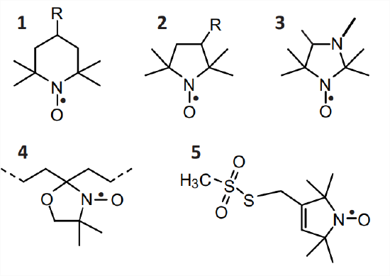
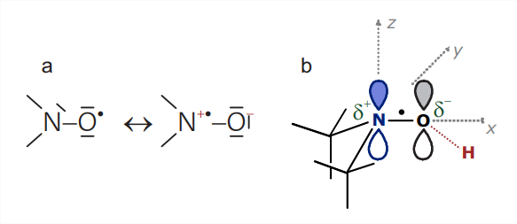
The nitroxide radical is defined by the \(\mathrm{N}-\mathrm{O}^{\bullet}\) group, which is isoelectronic with the carbonyl group \((\mathrm{C}=\mathrm{O})\) and can thus be replaced in approximate force field and molecular dynamics computations by a \(\mathrm{C}=\mathrm{O}\) group. The unpaired electron is distributed over both atoms, which contributes to radical stability, with a slight preference for the oxygen atom. Nitroxide radicals become stable on the time scale of months or years if both \(\alpha\) positions are sterically protected, for instance by attaching two methyl groups to each of the \(\alpha \mathrm{C}\) atoms (Fig. 10.1). Nitroxides of this type are thermally stable up to temperatures of about \(140^{\circ} \mathrm{C}\), but they are easily reduced to the corresponding hydroxylamines, for instance by ascorbic acid, and are unstable at very low and very high pH. Nitroxides with five-membered rings (structures \(\mathbf{2}, \boldsymbol{3}\), and \(\mathbf{5}\) ) tend to be chemically more stable than those with six-membered rings (6). The five-membered rings also have less conformational freedom than the six-membered rings.
Spin probes can be addressed to certain environments in heterogeneous systems by choice of appropriate substituents \(\mathrm{R}\) (Fig. 10.1). The unsubstituted species \((\mathrm{R}=\mathrm{H})\) are hydrophobic and partition preferably to nonpolar environments. Preference for hydrogen bond acceptors is achieved by hydroxyl derivatives \((\mathrm{R}=\mathrm{OH})\), whereas ionic environments can be addressed by a carboxylate group at sufficiently high \(\mathrm{pH}\left(\mathrm{R}=\mathrm{COO}^{-}\right)\)or by a trimethyl ammonium group \((\mathrm{R}=\) \(\left.\mathrm{N}\left(\mathrm{CH}_{3}\right)_{3}^{+}\right)\). Reactive groups \(\mathrm{R}\) are used for SDSL, such as the methanethiosulfonate group in the dehydro-PROXYL derivative MTSL 5, which selectively reacts with thiol groups under mild conditions. Thiol groups can be introduced into proteins by site-directed point mutation of an amino acid to cysteine and to RNA by replacement of a nucleobase by thiouridine. In DOXYL derivatives \(\mathbf{4}\), a six-membered ring is spiro-linked to an alkyl chain, which can be part of stearic acid or of lipid molecules. The \(\mathrm{N}^{\circ} \mathrm{O}^{\bullet}\) group in DOXYL derivatives is rigidly attached to the alkyl chain and nearly parallel to the axis of a hypothetical all-trans chain.
The nitroxide EPR spectrum
To a good approximation, the spin system of a nitroxide radical can be considered as an electron spin \(S=1 / 2\) coupled to the nuclear spin \(I=1\) of the \({ }^{14} \mathrm{~N}\) atom of the \(\mathrm{N}-\mathrm{O}^{\bullet}\) group. Hyperfine
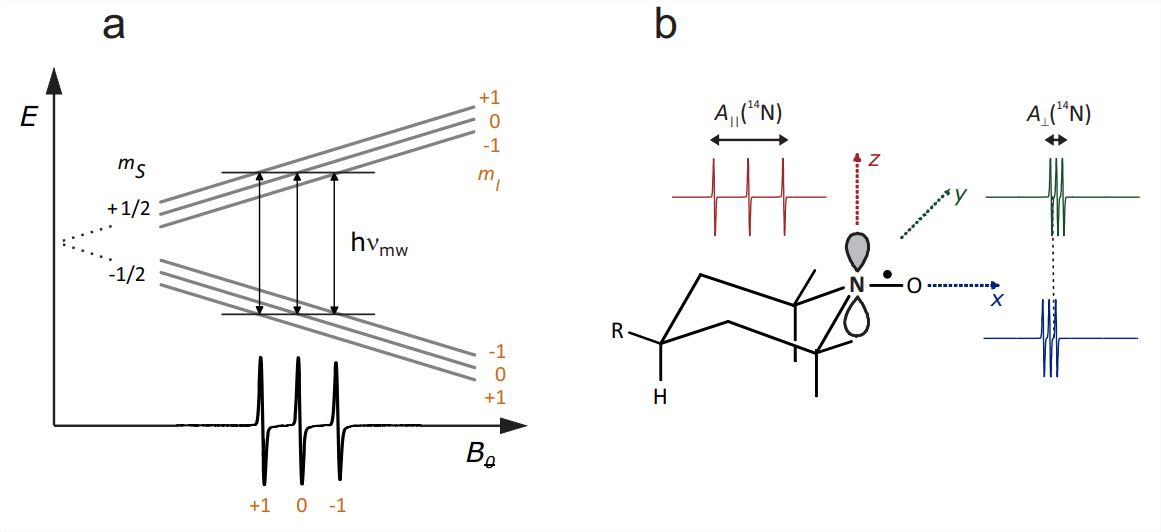
couplings to other nuclei, such as the methyl protons, are not usually resolved and contribute only to line broadening. The hyperfine coupling to the \(s p^{2}\) hybridized \({ }^{14} \mathrm{~N}\) atom has a significant isotropic Fermi contact contribution from spin density in the \(2 s\) orbital and a significant anisotropic contribution from spin density in the \(p_{\pi}\) orbital that combines with a \(p_{\pi}\) orbital on the oxygen atom to give the N-O bond partial double bond character. The direction of the lobes of the \(p_{\pi}\) orbital is chosen as the molecular \(z\) axis (Fig. 10.2(b)). The \({ }^{14} \mathrm{~N}\) hyperfine tensor has nearly axial symmetry with \(z\) being the unique axis. The hyperfine coupling is much larger along \(z\) (on the order of \(90 \mathrm{MHz}\) ) than in the \(x y\) plane (on the order of \(15 \mathrm{MHz}\) ).
The spin-orbit coupling, which induces \(g\) anisotropy, arises mainly at the \(\mathrm{O}\) atom, where a lone pair energy level is very close to the SOMO. The \(g\) tensor is orthorhombic with nearly maximal asymmetry. The largest \(g\) shift is positive and observed along the N-O bond, which is the molecular frame \(x\) axis \(\left(g_{x} \approx 2.009\right)\). An intermediate \(g\) shift is observed along the \(y\) axis \(\left(g_{y} \approx 2.006\right)\), whereas the \(g_{z}\) value is very close to \(g_{e}=2.0023\). At X-band frequencies, where \(\nu_{\mathrm{mw}} \approx 9.5 \mathrm{GHz}, g\) anisotropy corresponds to only \(1.13 \mathrm{mT}\) dispersion in resonance fields, while hyperfine anisotropy corresponds to \(6.5 \mathrm{mT}\) dispersion. At W-band frequencies, where \(\nu_{\mathrm{mw}} \approx 95 \mathrm{GHz}\), hyperfine anisotropy is still the same but \(g\) anisotropy contributes a ten times larger dispersion of \(11.3 \mathrm{mT}\), which now dominates.
The field-swept CW EPR spectrum for a single orientation can be understood by considering the selection rule that the magnetic quantum number \(m_{S}\) of the electron spin must change by 1 , whereas the magnetic quantum number \(m_{I}\) of the \({ }^{14} \mathrm{~N}\) nuclear spin must not change. Each transition can thus be assigned to a value of \(m_{I}\). For \(I=1\) there are three such values, \(m_{I}=-1,0\), and 1 (Fig. \(10.2(\mathrm{a})\) ). The microwave frequency \(\nu_{\mathrm{mw}}\) is fixed and resonance is observed at fields where the energy of the microwave quantum \(h \nu_{\mathrm{mw}}\) matches the energy of a transition.
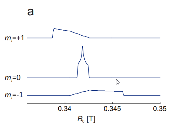
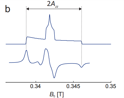
In order to construct the solid-state spectrum, orientation dependence of the three transitions must be considered (Fig. 10.3(a)). At each individual orientation, the \(m_{I}=0\) line is the center line. Since the hyperfine contributions scales with \(m_{I}\), it vanishes for this line and only \(g\) anisotropy is observed. At X band, where hyperfine anisotropy dominates by far, this line is the narrowest one. The lineshape is the one for pure \(g\) anisotropy (see Fig. 3.4). For \(m_{I}=+1\), the orientation with the largest \(g\) shift of the resonance field coincides with the one of smallest hyperfine shift. Hence, the smaller resonance field dispersion by \(g\) anisotropy subtracts from the larger dispersion by hyperfine anisotropy. For \(m_{I}=-1\), the situation is opposite and the two dispersions add. Hence, the \(m_{I}=-1\) transition, which at any given orientation is the high-field line, has the largest resonance dispersion, whereas the low-field \(m_{I}=+1\) transition has intermediate resonance field dispersion. The central feature in the total absorption spectrum (Fig. \(10.3(\mathrm{~b})\) ) is strongly dominated by the \(m_{I}=0\) transition, whereas the outer shoulders correspond to the \(m_{I}=+1\) (low field) and \(m_{I}=-1\) (high field) transitions at the \(z\) orientation. Therefore, the splitting between the outer extremities in the CW EPR spectrum, which correspond to these shoulders in the absorption spectrum, is \(2 A_{z z}\).
Influence of dynamics on the nitroxide spectrum
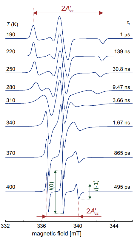
In liquid solution, molecules tumble stochastically due to Brownian rotational diffusion. In the following we consider isotropic rotational diffusion, where the molecule tumbles with the same average rate about any axis in its molecular frame. This is a good approximation for nitroxide spin probes with small substituents \(\mathrm{R}\). For instance, TEMPO \((\mathbf{1}\) with \(\mathrm{R}=\mathrm{H})\) is almost spherical with a van-der-Waals radius of \(3.43 \AA \AA\). In water at ambient temperature, the \(\tau_{\mathrm{r}}\) rotational correlation time for TEMPO is of the order of \(10 \mathrm{ps}\). The product \(\tau_{\mathrm{r}} \Delta \omega\) with the maximum anisotropy \(\Delta \omega\) of the nitroxide EPR spectrum on an angular frequency axis is much smaller than unity. In this situation, anisotropy averages and three narrow lines of equal width and intensity are expected. The spectrum in Fig. 10.2(a) corresponds to this situation and a closer look reveals that the high-field line has somewhat lower amplitude. This can be traced back to a larger linewidth than for the other two lines, which indicates a shorter \(T_{2}\) for the \(m_{I}=-1\) transition than for the other transitions. Indeed, transverse relaxation is dominated by the effect from combined hyperfine and \(g\) anisotropy, which is largest for the \(m_{I}=-1\) transition that has the largest anisotropic dispersion of resonance frequencies. With increasing rotational correlation time \(\tau_{r}\), one expects this relaxation process to become stronger, which should lead to more line broadening that is strongest for the high-field line and weakest for the central line. This is indeed observed in the simulation for \(\tau_{\mathrm{r}}=495\) ns shown in the bottom trace of Fig. \(10.4\).
According to Kivelson relaxation theory, the ratio of the line width of one of the outer lines to the line width of the central line is given by
\[\frac{T_{2}^{-1}\left(m_{I}\right)}{T_{2}^{-1}(0)}=1+B m_{I}+C m_{I}^{2}\]
where
\[B=-\frac{4}{15} b \Delta \gamma B_{0} T_{2}(0) \tau_{\mathrm{r}}\]
and
\[C=\frac{1}{8} b^{2} T_{2}(0) \tau_{\mathrm{r}}\]
with the hyperfine anisotropy parameter
\[b=\frac{4 \pi}{3}\left[A_{z z}-\frac{A_{x x}+A_{y y}}{2}\right]\]
and the electron Zeeman anisotropy parameter \(\Delta \gamma\)
\[\Delta \gamma=\frac{\mu_{\mathrm{B}}}{\hbar}\left[g_{z z}-\frac{g_{x x}+g_{y y}}{2}\right]\]
The relaxation time \(T_{2}(0)\) for the central line can be computed from the corresponding peak-topeak linewidth in field domain \(\Delta B_{p p}(0)\) as
\[T_{2}(0)=\frac{2}{\sqrt{3} g_{\text {iso }} \mu_{\mathrm{B}} \Delta B_{\mathrm{pp}}(0)}\]
Thus, Eqs. (10.1-10.3) can be solved for the only remaining unknown \(\tau_{\mathrm{r}}\). In practice, ratios of peak-to-peak line amplitudes \(I\left(m_{I}\right)\) are analyzed rather than linewidth ratios, as they can be measured with higher precision. The linewidth ratio is related to the amplitude ratio \(I(0) / I(-1)\) (see bottom trace in Fig. 10.4) in a first derivative spectrum by
\[\frac{T_{2}^{-1}\left(m_{I}\right)}{T_{2}^{-1}(0)}=\sqrt{\frac{I(0)}{I\left(m_{I}\right)}}\]
since the integral intensity of the absorption line (double integral of the derivative lineshape) is the same for each of the three transitions. The rotational correlation time can thus be determined by, e.g.,
\[\tau_{\mathrm{r}}=\frac{\sqrt{3}}{2 b}\left[\frac{b}{8}-\frac{4 \Delta \gamma B_{0}}{15}\right]^{-1} \frac{g_{\mathrm{iso}} \mu_{\mathrm{B}}}{\hbar} \Delta B_{\mathrm{pp}}(0)\left[\sqrt{\frac{I(0)}{I(-1)}}-1\right]\]
where \(\Delta B_{0}\) is the peak-to-peak linewidth of the central line. This equation can be applied in the fast tumbling regime, where the three individual lines for \(m_{I}=-1,0\), and \(+1\) can still be clearly recognized and have the shape of symmetric derivative absorption lines.
For slower tumbling with \(\tau_{\mathrm{r}}>1.5 \mathrm{~ns}\), the line shape becomes more complex and approaches the rigid limit (solid-state spectrum) at about \(\tau_{\mathrm{r}}=1 \mu \mathrm{s}\) (Fig. 10.4). These lineshapes can be simulated by considering multi-site exchange between different orientations of the molecule with respect to the magnetic field. Unlike for two-site exchange, which is discussed in the NMR part of the lecture course (see Section 3 of the NMR lecture notes), no closed expressions can be obtained for multi-site exchange. Nevertheless we can estimate the time scale where the spectral features are broadest and transverse relaxation times are shortest. Coalescence for two-site exchange is observed at \(\Delta \Omega / k=2 \sqrt{2}\). By substituting \(k\) by \(1 / \tau_{\text {r and }} \Delta \Omega\) by the maximum anisotropy of \(7.6 \mathrm{mT}\), corresponding to \(213 \mathrm{MHz}\), we find a "coalescence time" \(2 \sqrt{2} / \Delta \Omega \approx 2.1\) ns. The simulations in Fig. \(10.4\) show indeed that around this rotational correlation time, the

character of the spectrum changes from fast orientation exchange (liquid-like spectrum with three distinct peaks) to slow orientation exchange (solid-like spectrum).
A simple way of analyzing a temperature dependence, such as the one shown in Fig. 10.4, is to plot the outer extrema separation \(2 A_{z z}^{\prime}\) as a function of temperature (Fig. 10.5). The "coalescence time" in such a plot corresponds to the largest gradient \(\mathrm{d} A_{z z}^{\prime} / \mathrm{d} T\), which coincides with the mean between the \(2 A_{z z}^{\prime}\) values in the fast tumbling limit and rigid limit, which is \(5 \mathrm{mT}\). In the case at hand, this coalescence time is \(3.5 \mathrm{~ns}\) and is observed at a temperature \(T_{5 \mathrm{mT}}=312\) \(\mathrm{K}\). The \(T_{5 \mathrm{mT}}\) temperature is the temperature where the material becomes "soft" and molecular conformations can rearrange. Nitroxide spectra in the slow tumbling regime can reveal more details on dynamics, for instance, whether there are preferred rotation axes, whether motion is restricted due to covalent linkage of the nitroxide to a large molecule, or whether there is local order, such as in a lipid bilayer.
Polarity and proticity
Delocalization of the unpaired electron in the \(\mathrm{N}-\mathrm{O}^{\bullet}\) group can be understood by considering mesomeric structures (Fig. 10.6). If the unpaired electron resides on oxygen, the formal number of valence electrons is five on nitrogen and six on oxygen, corresponding to the nuclear charge that is not compensated by inner shell electrons. Hence, both atoms are formally neutral in this limiting structure. If, on the other hand, the unpaired electron resides on the nitrogen atom, only four valence electrons are assigned to this atom, whereas seven valence electrons are assigned to the oxygen atom. This corresponds to charge separation with the formal positive charge on nitrogen and the formal negative charge on oxygen. The charge-separated form is favored in polar solvents, which screen Coulomb attraction between the two charges, whereas the neutral form is favored in nonpolar solvents. Hence, for a given nitroxide radical in a series of solvents, the \({ }^{14} \mathrm{~N}\) hyperfine coupling, which stems from spin density on the nitrogen atom, is expected to increase with increasing solvent polarity. This effect has indeed been found. It is most easily seen in the solid state for \(A_{z z}\) but can also be discerned in the liquid state for \(A_{\text {iso }}\).
The change in \(A_{z z}\) is expected to be anti-correlated to the \(g_{x x}\) shift, because this shift arises from SOC at the oxygen atom and, the higher spin density on the nitrogen atom is, the lower it is on the oxygen atom. This effect has also been found and is most easily detected by high-field/high-frequency EPR at frequencies of W-band frequencies of \(\approx 95 \mathrm{GHz}\) or even higher frequencies. How \(A_{z z}\) is correlated to \(g_{x x}\) depends on proticity of the solvent. Protic solvents form hydrogen bonds with the lone pairs on the oxygen atom of the N-O \({ }^{\bullet}\) group. This lowers energy of the lone pair orbitals, making excitation of an electron from these orbitals to the SOMO less likely. Since this excitation provides the main contribution to SOC and thus to \(g_{x x}\) shift, hydrogen bonding to oxygen reduces \(g_{x x}\) shift. If two nitroxides have the same hyperfine coupling \(A_{z z}\) in an aprotic and protic environment, \(g_{x x}\) will be lower in the protic environment. This effect has also been found. In some cases it was possible to discern nitroxide labels with zero, one, and two hydrogen bonds by resolution of their \(g_{x x}\) features in W-band CW EPR spectra. Slopes of \(-1.35 \mathrm{~T}^{-1}\) for aprotic at \(-2 \mathrm{~T}^{-1}\) for protic environments have been found for the correlation between \(A_{z z}\) and \(g_{x x}\) for MTSL in spin-labeled bacteriorhodopsin in lipid bilayers [Ste+00].
Water accessibility
Polarity and proticity are proxy parameters for water accessibility of spin-labeled sites in proteins. Two other techniques provide complementary information. First, water can be replaced by deuterated water and the modulation depth of deuterium ESEEM can be measured. Because of the \(r^{-6}\) dependence of modulation depth (see Eq. (8.7)) the technique is most sensitive to deuterium nuclei in the close vicinity of the spin label. As long as \(k \ll 1\), modulation depth contributions of individual nuclei add, so that the total deuterium modulation depth is a measure for local deuterium concentration close to the label. Data can be processed in a way that removes the contribution from directly hydrogen-bonded nuclei. Strictly speaking, this technique measures the concentration of not only water protons but also the one of any exchangeable protons near the label, but only to the extent that these exchangeable protons are water accessible during sample preparation or measurement.
A second, more direct technique that is applicable at ambient temperature measures the proton NMR signal as a function of irradiated microwave power with the microwave frequency being on-resonant with the central transition of a nitroxide spin label. Such irradiation transfers electron spin polarization to water protons by the Overhauser effect. This Overhauser dynamic nuclear polarization (DNP) is highly specific to water, as it critically depends on the water proton NMR signal being narrow and on fast diffusion of water. In biomolecules, water accessibility of spin labels is high at water-exposed surfaces of soluble and membrane proteins and low inside the proteins and at lipid-exposed surfaces. For transporters, water accessibility can change with state in the transport process.
Oxygen accessibility
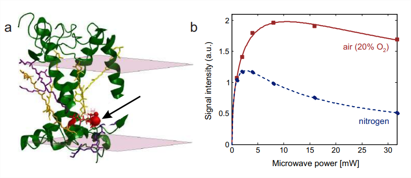
Since collision of paramagnetic triplet oxygen with spin probes enhances relaxation (Fig. \(7.4)\), the saturation parameter \(S=\omega_{1}^{2} T_{1} T 2\) is smaller for oxygen-accessible spin labels than for spin labels not accessible to oxygen. This change can be detected by CW progressive power saturation measurements (Section 7.2.2). The experiment is most conveniently performed with capillary tubes made of the gas permeable plastic TPX. A reference measurement is performed in a nitrogen atmosphere, which causes deoxygenation of the sample on the time scale of 15 min. The gas stream is then changed to air (20% oxygen) or pure oxygen and the measurement is repeated. Such data are shown in Fig. \(10.7\) for residue 229 in major plant light harvesting complex LHCII. This residue is lipid exposed. As a nonpolar molecule, oxygen dissolves well in the alkyl chain region of a lipid bilayer. Accordingly, the signal saturates at higher power in an air atmosphere than in a nitrogen atmosphere. Oxygen accessibility can be quantified by a normalized \(P_{1 / 2}\) parameter (Section 7.2.2).
Local pH measurements
The \({ }^{14} \mathrm{~N}\) hyperfine coupling of nitroxide spin probes becomes \(\mathrm{pH}\) sensitive if the heterocycle that contains the \(\mathrm{N}-\mathrm{O}^{\bullet}\) group also contains a nitrogen atom that can be protonated in the desired \(\mathrm{pH}\) range. This applies, for instance, to the imidazolidine nitroxide 3 in Fig. \(10.1\), which has a pK value of \(\approx 4.7\) and exhibits a change in isotropic \({ }^{14}\) N hyperfine coupling of \(0.13 \mathrm{mT}\) between the protonated (1.43 mT) and deprotonated \((1.56 \mathrm{mT})\) form, which can be resolved easily in liquid solution. By modifying the probe to a label, local \(\mathrm{pH}\) can be measured near a residue of interest in a protein.