11.2: The Advancement and Molar Reaction Quantities

\( \newcommand{\tx}[1]{\text{#1}}      % text in math mode\)
 \( \newcommand{\subs}[1]{_{\text{#1}}} % subscript text\)
 \( \newcommand{\sups}[1]{^{\text{#1}}} % superscript text\)
 \( \newcommand{\st}{^\circ}            % standard state symbol\)
 \( \newcommand{\id}{^{\text{id}}}      % ideal\)
 \( \newcommand{\rf}{^{\text{ref}}}     % reference state\)
 \( \newcommand{\units}[1]{\mbox{$\thinspace$#1}}\)
 \( \newcommand{\K}{\units{K}}  % kelvins\)
 \( \newcommand{\degC}{^\circ\text{C}} % degrees Celsius\)
 \( \newcommand{\br}{\units{bar}}  % bar (\bar is already defined)\)
 \( \newcommand{\Pa}{\units{Pa}}\)
 \( \newcommand{\mol}{\units{mol}}  % mole\)
 \( \newcommand{\V}{\units{V}}  % volts\)
 \( \newcommand{\timesten}[1]{\mbox{$\,\times\,10^{#1}$}}\)
 \( \newcommand{\per}{^{-1}}  % minus one power\)
 \( \newcommand{\m}{_{\text{m}}}  % subscript m for molar quantity\)
 \( \newcommand{\CVm}{C_{V,\text{m}}} % molar heat capacity at const.V\)
 \( \newcommand{\Cpm}{C_{p,\text{m}}} % molar heat capacity at const.p\)
 \( \newcommand{\kT}{\kappa_T} % isothermal compressibility\)
 \( \newcommand{\A}{_{\text{A}}}  % subscript A for solvent or state A\)
 \( \newcommand{\B}{_{\text{B}}}  % subscript B for solute or state B\)
 \( \newcommand{\bd}{_{\text{b}}}  % subscript b for boundary or boiling point\)
 \( \newcommand{\C}{_{\text{C}}}  % subscript C\)
 \( \newcommand{\f}{_{\text{f}}}  % subscript f for freezing point\)
 \( \newcommand{\mA}{_{\text{m},\text{A}}} % subscript m,A (m=molar)\)
 \( \newcommand{\mB}{_{\text{m},\text{B}}} % subscript m,B (m=molar)\)
 \( \newcommand{\mi}{_{\text{m},i}}        % subscript m,i (m=molar)\)
 \( \newcommand{\fA}{_{\text{f},\text{A}}} % subscript f,A (for fr. pt.)\)
 \( \newcommand{\fB}{_{\text{f},\text{B}}} % subscript f,B (for fr. pt.)\)
 \( \newcommand{\xbB}{_{x,\text{B}}}       % x basis, B\)
 \( \newcommand{\xbC}{_{x,\text{C}}}       % x basis, C\)
 \( \newcommand{\cbB}{_{c,\text{B}}}       % c basis, B\)
 \( \newcommand{\mbB}{_{m,\text{B}}}       % m basis, B\)
 \( \newcommand{\kHi}{k_{\text{H},i}}      % Henry's law constant, x basis, i\)
 \( \newcommand{\kHB}{k_{\text{H,B}}}      % Henry's law constant, x basis, B\)
 \( \newcommand{\arrow}{\,\rightarrow\,} % right arrow with extra spaces\)
 \( \newcommand{\arrows}{\,\rightleftharpoons\,} % double arrows with extra spaces\)
 \( \newcommand{\ra}{\rightarrow} % right arrow (can be used in text mode)\)
 \( \newcommand{\eq}{\subs{eq}} % equilibrium state\)
 \( \newcommand{\onehalf}{\textstyle\frac{1}{2}\D} % small 1/2 for display equation\)
 \( \newcommand{\sys}{\subs{sys}} % system property\)
 \( \newcommand{\sur}{\sups{sur}} % surroundings\)
 \( \renewcommand{\in}{\sups{int}} % internal\)
 \( \newcommand{\lab}{\subs{lab}} % lab frame\)
 \( \newcommand{\cm}{\subs{cm}} % center of mass\)
 \( \newcommand{\rev}{\subs{rev}} % reversible\)
 \( \newcommand{\irr}{\subs{irr}} % irreversible\)
 \( \newcommand{\fric}{\subs{fric}} % friction\)
 \( \newcommand{\diss}{\subs{diss}} % dissipation\)
 \( \newcommand{\el}{\subs{el}} % electrical\)
 \( \newcommand{\cell}{\subs{cell}} % cell\)
 \( \newcommand{\As}{A\subs{s}} % surface area\)
 \( \newcommand{\E}{^\mathsf{E}} % excess quantity (superscript)\)
 \( \newcommand{\allni}{\{n_i \}} % set of all n_i\)
 \( \newcommand{\sol}{\hspace{-.1em}\tx{(sol)}}\)
 \( \newcommand{\solmB}{\tx{(sol,$\,$$m\B$)}}\)
 \( \newcommand{\dil}{\tx{(dil)}}\)
 \( \newcommand{\sln}{\tx{(sln)}}\)
 \( \newcommand{\mix}{\tx{(mix)}}\)
 \( \newcommand{\rxn}{\tx{(rxn)}}\)
 \( \newcommand{\expt}{\tx{(expt)}}\)
 \( \newcommand{\solid}{\tx{(s)}}\)
 \( \newcommand{\liquid}{\tx{(l)}}\)
 \( \newcommand{\gas}{\tx{(g)}}\)
 \( \newcommand{\pha}{\alpha}        % phase alpha\)
 \( \newcommand{\phb}{\beta}         % phase beta\)
 \( \newcommand{\phg}{\gamma}        % phase gamma\)
 \( \newcommand{\aph}{^{\alpha}}     % alpha phase superscript\)
 \( \newcommand{\bph}{^{\beta}}      % beta phase superscript\)
 \( \newcommand{\gph}{^{\gamma}}     % gamma phase superscript\)
 \( \newcommand{\aphp}{^{\alpha'}}   % alpha prime phase superscript\)
 \( \newcommand{\bphp}{^{\beta'}}    % beta prime phase superscript\)
 \( \newcommand{\gphp}{^{\gamma'}}   % gamma prime phase superscript\)
 \( \newcommand{\apht}{\small\aph} % alpha phase tiny superscript\)
 \( \newcommand{\bpht}{\small\bph} % beta phase tiny superscript\)
 \( \newcommand{\gpht}{\small\gph} % gamma phase tiny superscript\)

\( \newcommand{\upOmega}{\Omega}\)

 \( \newcommand{\dif}{\mathop{}\!\mathrm{d}}   % roman d in math mode, preceded by space\)
 \( \newcommand{\Dif}{\mathop{}\!\mathrm{D}}   % roman D in math mode, preceded by space\)
 \( \newcommand{\df}{\dif\hspace{0.05em} f} % df\)

 \(\newcommand{\dBar}{\mathop{}\!\mathrm{d}\hspace-.3em\raise1.05ex{\Rule{.8ex}{.125ex}{0ex}}} % inexact differential \)
 \( \newcommand{\dq}{\dBar q} % heat differential\)
 \( \newcommand{\dw}{\dBar w} % work differential\)
 \( \newcommand{\dQ}{\dBar Q} % infinitesimal charge\)
 \( \newcommand{\dx}{\dif\hspace{0.05em} x} % dx\)
 \( \newcommand{\dt}{\dif\hspace{0.05em} t} % dt\)
 \( \newcommand{\difp}{\dif\hspace{0.05em} p} % dp\)
 \( \newcommand{\Del}{\Delta}\)
 \( \newcommand{\Delsub}[1]{\Delta_{\text{#1}}}\)
 \( \newcommand{\pd}[3]{(\partial #1 / \partial #2 )_{#3}} % \pd{}{}{} - partial derivative, one line\)
 \( \newcommand{\Pd}[3]{\left( \dfrac {\partial #1} {\partial #2}\right)_{#3}} % Pd{}{}{} - Partial derivative, built-up\)
 \( \newcommand{\bpd}[3]{[ \partial #1 / \partial #2 ]_{#3}}\)
 \( \newcommand{\bPd}[3]{\left[ \dfrac {\partial #1} {\partial #2}\right]_{#3}}\)
 \( \newcommand{\dotprod}{\small\bullet}\)
 \( \newcommand{\fug}{f} % fugacity\)
 \( \newcommand{\g}{\gamma} % solute activity coefficient, or gamma in general\)
 \( \newcommand{\G}{\varGamma} % activity coefficient of a reference state (pressure factor)\)
 \( \newcommand{\ecp}{\widetilde{\mu}} % electrochemical or total potential\)
 \( \newcommand{\Eeq}{E\subs{cell, eq}} % equilibrium cell potential\)
 \( \newcommand{\Ej}{E\subs{j}} % liquid junction potential\)
 \( \newcommand{\mue}{\mu\subs{e}} % electron chemical potential\)
\( \newcommand{\defn}{\,\stackrel{\mathrm{def}}{=}\,} % "equal by definition" symbol\)

 \( \newcommand{\D}{\displaystyle} % for a line in built-up\)
 \( \newcommand{\s}{\smash[b]} % use in equations with conditions of validity\)
 \( \newcommand{\cond}[1]{\\[-2.5pt]{}\tag*{#1}}\)
 \( \newcommand{\nextcond}[1]{\\[-5pt]{}\tag*{#1}}\)
 \( \newcommand{\R}{8.3145\units{J$\,$K$\per\,$mol$\per$}}     % gas constant value\)
 \( \newcommand{\Rsix}{8.31447\units{J$\,$K$\per\,$mol$\per$}} % gas constant value - 6 sig figs\)

\( \newcommand{\jn}{\hspace3pt\lower.3ex{\Rule{.6pt}{2ex}{0ex}}\hspace3pt} \)
\( \newcommand{\ljn}{\hspace3pt\lower.3ex{\Rule{.6pt}{.5ex}{0ex}}\hspace-.6pt\raise.45ex{\Rule{.6pt}{.5ex}{0ex}}\hspace-.6pt\raise1.2ex{\Rule{.6pt}{.5ex}{0ex}} \hspace3pt} \)
\( \newcommand{\lljn}{\hspace3pt\lower.3ex{\Rule{.6pt}{.5ex}{0ex}}\hspace-.6pt\raise.45ex{\Rule{.6pt}{.5ex}{0ex}}\hspace-.6pt\raise1.2ex{\Rule{.6pt}{.5ex}{0ex}}\hspace1.4pt\lower.3ex{\Rule{.6pt}{.5ex}{0ex}}\hspace-.6pt\raise.45ex{\Rule{.6pt}{.5ex}{0ex}}\hspace-.6pt\raise1.2ex{\Rule{.6pt}{.5ex}{0ex}}\hspace3pt} \) 

Many of the processes of interest to chemists can be described by balanced reaction equations, or chemical equations, for the conversion of reactants into products. Thus, for the vaporization of water we write \[ \ce{H2O}\tx{(l)} \arrow \ce{H2O}\tx{(g)} \] For the dissolution of sodium chloride in water, we write \[ \ce{NaCl}\tx{(s)} \arrow \ce{Na+}\tx{(aq)} + \ce{Cl-}\tx{(aq)} \] For the Haber synthesis of ammonia, the reaction equation can be written \begin{equation*} \ce{N2}\tx{(g)} + \ce{3H2}\tx{(g)} \arrow \ce{2NH3}\tx{(g)} \end{equation*}

The essential feature of a reaction equation is that equal amounts of each element and equal net charges appear on both sides; the equation is said to be balanced. Thus, matter and charge are conserved during the process, and the process can take place in a closed system. The species to the left of a single arrow are called reactants, the species to the right are called products, and the arrow indicates the forward direction of the process.

A reaction equation is sometimes written with right and left arrows \[ \ce{N2}\tx{(g)} + \ce{3H2}\tx{(g)} \arrows \ce{2NH3}\tx{(g)} \] to indicate that the process is at reaction equilibrium. It can also be written as a stoichiometric equation with an equal sign: \[ \ce{N2}\tx{(g)} + \ce{3H2}\tx{(g)} = \ce{2NH3}\tx{(g)} \]

A reaction equation shows stoichiometric relations among the reactants and products. It is important to keep in mind that it specifies neither the initial and final states of a chemical process, nor the change in the amount of a reactant or product during the process. For example, the reaction equation N\(_2\) + 3 H\(_2\) \(\ra\) 2 NH\(_3\) does not imply that the system initially contains only N\(_2\) and H\(_2\), or that only NH\(_3\) is present in the final state; and it does not mean that the process consists of the conversion of exactly one mole of N\(_2\) and three moles of H\(_2\) to two moles of NH\(_3\) (although this is a possibility). Instead, the reaction equation tells us that a change in the amount of N\(_2\) is accompanied by three times this change in the amount of H\(_2\) and by twice this change, with the opposite sign, in the amount of NH\(_3\).

11.2.1 An example: ammonia synthesis

It is convenient to indicate the progress of a chemical process with a variable called the advancement. The reaction equation
N\(_2\) + 3 H\(_2\) \(\ra\) 2 NH\(_3\) for the synthesis of ammonia synthesis will serve to illustrate this concept. Let the system be a gaseous mixture of N\(_2\), H\(_2\), and NH\(_3\).

If the system is open and the intensive properties remain uniform throughout the gas mixture, there are five independent variables. We can choose them to be \(T\), \(p\), and the amounts of the three substances. We can write the total differential of the enthalpy, for instance, as \begin{equation} \begin{split} \dif H & = \Pd{H}{T}{p,\allni}\dif T + \Pd{H}{p}{T,\allni}\difp \cr & \quad + H\subs{N\(_2\)}\dif n\subs{N\(_2\)} + H\subs{H\(_2\)}\dif n\subs{H\(_2\)} + H\subs{NH\(_3\)}\dif n\subs{NH\(_3\)} \end{split} \tag{11.2.1} \end{equation} The notation \(\allni\) stands for the set of amounts of all substances in the mixture, and the quantities \(H\subs{N\(_2\)}\), \(H\subs{H\(_2\)}\), and \(H\subs{NH\(_3\)}\) are partial molar enthalpies. For example, \(H\subs{N\(_2\)}\) is defined by \begin{equation} H\subs{N\(_2\)} = \Pd{H}{n\subs{N\(_2\)}}{T, p, n\subs{H\(_2\)}, n\subs{NH\(_3\)}} \tag{11.2.2} \end{equation}

If the system is closed, the amounts of the three substances can still change because of the reaction N\(_2\) + 3 H\(_2\) \(\ra\) 2 NH\(_3\), and the number of independent variables is reduced from five to three. We can choose them to be \(T\), \(p\), and a variable called advancement.

The advancement (or extent of reaction), \(\xi\), is the amount by which the reaction defined by the reaction equation has advanced in the forward direction from specified initial conditions. The quantity \(\xi\) has dimensions of amount of substance, the usual unit being the mole.

Let the initial amounts be \(n_{\tx{N}_2,0}\), \(n_{\tx{H}_2,0}\), and \(n_{\tx{NH}_3,0}\). Then at any stage of the reaction process in the closed system, the amounts are given by \begin{equation} n\subs{N\(_2\)} = n_{\tx{N}_2,0} - \xi \qquad n\subs{H\(_2\)} = n_{\tx{H}_2,0} - 3\xi \qquad n\subs{NH\(_3\)} = n_{\tx{NH}_3,0} + 2\xi \tag{11.2.3} \end{equation} These relations come from the stoichiometry of the reaction as expressed by the stoichiometric coefficients in the reaction equation. The second relation, for example, expresses the fact that when one mole of reaction has occurred (\(\xi=1\mol\)), the amount of H\(_2\) in the closed system has decreased by three moles.

Taking the differentials of Eqs. 11.2.3, we find that infinitesimal changes in the amounts are related to the change of \(\xi\) as follows: \begin{equation} \dif n\subs{N\(_2\)} = - \dif\xi \qquad \dif n\subs{H\(_2\)} = - 3\dif\xi \qquad \dif n\subs{NH\(_3\)} = 2\dif\xi \tag{11.2.4} \end{equation} These relations show that in a closed system, the changes in the various amounts are not independent. Substitution in Eq. 11.2.1 of the expressions for \(\dif n\subs{N\(_2\)}\), \(\dif n\subs{H\(_2\)}\), and \(\dif n\subs{NH\(_3\)}\) gives \begin{gather} \s{ \begin{split} \dif H & = \Pd{H}{T}{p, \xi}\dif T + \Pd{H}{p}{T, \xi}\difp \cr & \quad + \left( -H\subs{N\(_2\)} - 3H\subs{H\(_2\)} + 2H\subs{NH\(_3\)} \right)\dif\xi \end{split} } \tag{11.2.5} \cond{(closed system)} \end{gather} (The subscript \(\allni\) on the partial derivatives has been replaced by \(\xi\) to indicate the same thing: that the derivative is taken with the amount of each species held constant.)

Equation 11.2.5 gives an expression for the total differential of the enthalpy with \(T\), \(p\), and \(\xi\) as the independent variables. The coefficient of \(\dif \xi\) in this equation is called the molar reaction enthalpy, or molar enthalpy of reaction, \(\Delsub{r}H\): \begin{equation} \Delsub{r}H = -H\subs{N\(_2\)} - 3H\subs{H\(_2\)} + 2H\subs{NH\(_3\)} \tag{11.2.6} \end{equation} We identify this coefficient as the partial derivative \begin{equation} \Delsub{r}H = \Pd{H}{\xi}{T, p} \tag{11.2.7} \end{equation} That is, the molar reaction enthalpy is the rate at which the enthalpy changes with the advancement as the reaction proceeds in the forward direction at constant \(T\) and \(p\).

The partial molar enthalpy of a species is the enthalpy change per amount of the species added to an open system. To see why the particular combination of partial molar enthalpies on the right side of Eq. 11.2.6 is the rate at which enthalpy changes with advancement in the closed system, we can imagine the following process at constant \(T\) and \(p\): An infinitesimal amount \(\dif n\) of N\(_2\) is removed from an open system, three times this amount of H\(_2\) is removed from the same system, and twice this amount of NH\(_3\) is added to the system. The total enthalpy change in the open system is \(\dif H = (-H\subs{N\(_2\)} - 3H\subs{H\(_2\)} + 2H\subs{NH\(_3\)})\dif n\). The net change in the state of the system is equivalent to an advancement \(\dif\xi = \dif n\) in a closed system, so \(\dif H/\dif\xi\) in the closed system is equal to \((-H\subs{N\(_2\)} - 3H\subs{H\(_2\)} + 2H\subs{NH\(_3\)})\) in agreement with Eqs. 11.2.6 and 11.2.7.

Note that because the advancement is defined by how we write the reaction equation, the value of \(\Delsub{r}H\) also depends on the reaction equation. For instance, if we change the reaction equation for ammonia synthesis from N\(_2\) + 3 H\(_2\) \(\ra\) 2 NH\(_3\) to \[ \ce{1/2N2} + \ce{3/2H2} \arrow \ce{NH3} \] then the value of \(\Delsub{r}H\) is halved.

11.2.2 Molar reaction quantities in general

Now let us generalize the relations of the preceding section for any chemical process in a closed system. Suppose the stoichiometric equation has the form \begin{equation} a\tx{A} + b\tx{B} = d\tx{D} + e\tx{E} \tag{11.2.8} \end{equation} where A and B are reactant species, D and E are product species, and \(a\), \(b\), \(d\), and \(e\) are the corresponding stoichiometric coefficients. We can rearrange this equation to \begin{equation} 0 = - a\tx{A} - b\tx{B} + d\tx{D} + e\tx{E} \tag{11.2.9} \end{equation}

In general, the stoichiometric relation for any chemical process is \begin{equation} 0 = \sum_i\nu_i \tx{A}_i \tag{11.2.10} \end{equation} where \(\nu_i\) is the stoichiometric number of species A\(_i\), a dimensionless quantity taken as negative for a reactant and positive for a product. In the ammonia synthesis example of the previous section, the stoichiometric relation is \(0 = -\tx{N}_2 - 3\tx{H}_2 + 2\tx{NH}_3\) and the stoichiometric numbers are \(\nu\subs{N\(_2\)} = -1\), \(\nu\subs{H\(_2\)} = -3\), and \(\nu\subs{NH\(_3\)} = +2\). In other words, each stoichiometric number is the same as the stoichiometric coefficient in the reaction equation, except that the sign is negative for a reactant.

The amount of reactant or product species \(i\) present in the closed system at any instant depends on the advancement at that instant, and is given by \begin{gather} \s{ n_i = n_{i,0} + \nu_i\xi } \tag{11.2.11} \cond{(closed system)} \end{gather} The infinitesimal change in the amount due to an infinitesimal change in the advancement is \begin{gather} \s{ \dif n_i = \nu_i\dif\xi } \tag{11.2.12} \cond{(closed system)} \end{gather}

In an open system, the total differential of extensive property \(X\) is \begin{equation} \dif X = \Pd{X}{T}{p, \allni}\dif T + \Pd{X}{p}{T, \allni}\difp + \sum_i X_i\dif n_i \tag{11.2.13} \end{equation} where \(X_i\) is a partial molar quantity. We restrict the system to a closed one with \(T\), \(p\), and \(\xi\) as the independent variables. Then, with the substitution \(\dif n_i = \nu_i\dif\xi\) from Eq. 11.2.12, the total differential of \(X\) becomes \begin{gather} \s{ \dif X = \Pd{X}{T}{p, \xi}\dif T + \Pd{X}{p}{T, \xi}\difp + \Delsub{r}X\dif\xi } \tag{11.2.14} \cond{(closed system)} \end{gather} where the coefficient \(\Delsub{r}X\) is the molar reaction quantity defined by \begin{equation} \Delsub{r}X \defn \sum_i\nu_i X_i \tag{11.2.15} \end{equation} Equation 11.2.14 allows us to identify the molar reaction quantity as a partial derivative: \begin{gather} \s{ \Delsub{r}X = \Pd{X}{\xi}{T, p} } \tag{11.2.16} \cond{(closed system)} \end{gather}

It is important to observe the distinction between the notations \(\Del X\), the finite change of \(X\) during a process, and \(\Delsub{r}X\), a differential quantity that is a property of the system in a given state. The fact that both notations use the symbol \(\Del\) can be confusing. Equation 11.2.16 shows that we can think of \(\Delsub{r}\) as an operator.

In dealing with the change of an extensive property \(X\) as \(\xi\) changes, we must distinguish between molar integral and molar differential reaction quantities.

 

• \(\Del X/\Del\xi\) is a molar integral reaction quantity, the ratio of two finite differences between the final and initial states of a process. These states are assumed to have the same temperature and the same pressure. This e-book will use a notation such as \(\Del H\m\rxn\) for a molar integral reaction enthalpy: \begin{gather} \s{ \Del H\m\rxn = \frac{\Del H\rxn}{\Del\xi} = \frac{H(\xi_2)-H(\xi_1)}{\xi_2 - \xi_1} } \tag{11.2.17} \cond{(\(T_2{=}T_1,p_2{=}p_1\))} \end{gather}

   

• \(\Delsub{r}X\) is a molar differential reaction quantity. Equation 11.2.16 shows that \(\Delsub{r}X\) is the rate at which the extensive property \(X\) changes with the advancement in a closed system at constant \(T\) and \(p\). The value of \(\Delsub{r}X\) is in general a function of the independent variables \(T\), \(p\), and \(\xi\).

   

The notation for a molar differential reaction quantity such as \(\Delsub{r}H\) includes a subscript following the \(\Del\) symbol to indicate the kind of chemical process. The subscript “r” denotes a reaction or process in general. The meanings of “vap,” “sub,” “fus,” and “trs” were described in Sec. 8.3.1. Subscripts for specific kinds of reactions and processes are listed in Sec. D.2 of Appendix D and are illustrated in sections to follow.

For certain kinds of processes, it may happen that a partial molar quantity \(X_i\) remains constant for each species \(i\) as the process advances at constant \(T\) and \(p\). If \(X_i\) remains constant for each \(i\), then according to Eq. 11.2.15 the value of \(\Delsub{r}X\) must also remain constant as the process advances. Since \(\Delsub{r}X\) is the rate at which \(X\) changes with \(\xi\), in such a situation \(X\) is a linear function of \(\xi\). This means that the molar integral reaction quantity \(\Del X\m\rxn\) defined by \(\Del X/\Del\xi\) is equal, for any finite change of \(\xi\), to \(\Delsub{r}X\).

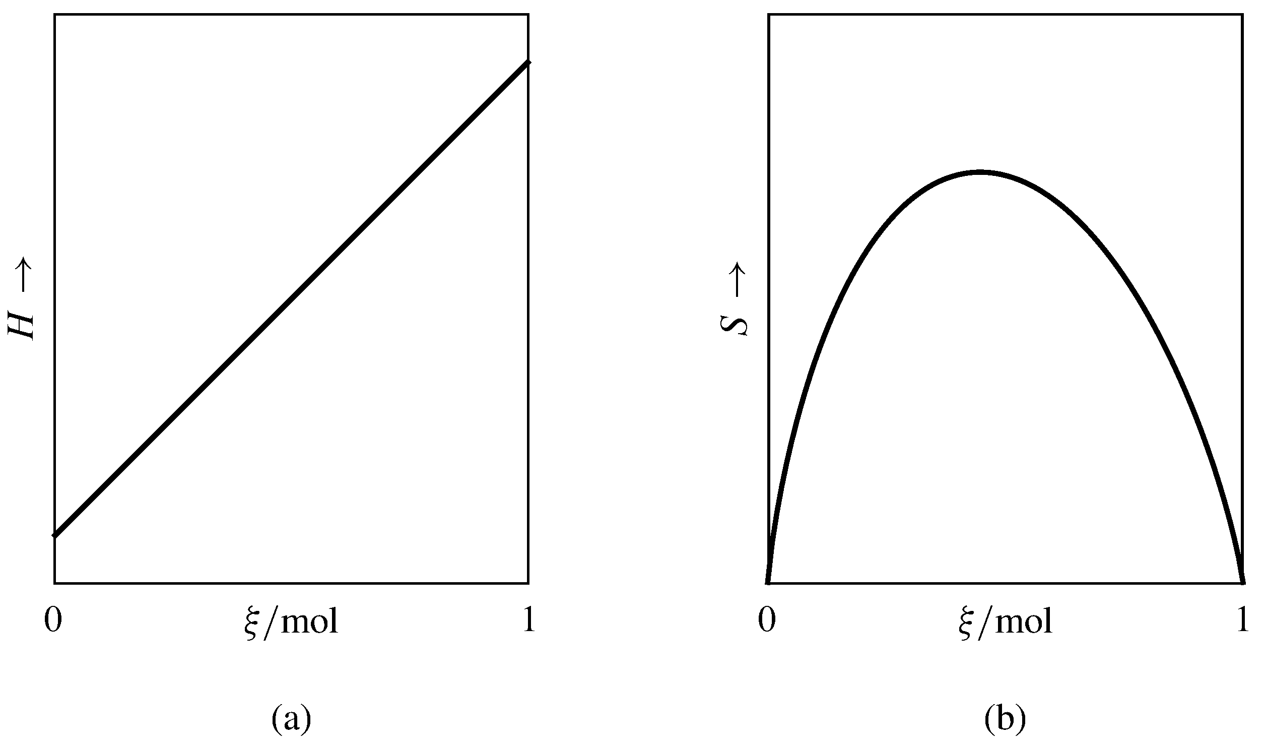
Figure 11.6 Enthalpy and entropy as functions of advancement at constant \(T\) and \(p\). The curves are for a reaction A\(\rightarrow\)2B with positive \(\Delsub{r}H\) taking place in an ideal gas mixture with initial amounts \(n_{\tx{A},0}=1\mol\) and \(n_{\tx{B},0}=0\).

An example is the partial molar enthalpy \(H_i\) of a constituent of an ideal gas mixture, an ideal condensed-phase mixture, or an ideal-dilute solution. In these ideal mixtures, \(H_i\) is independent of composition at constant \(T\) and \(p\) (Secs. 9.3.3, 9.4.3, and 9.4.7). When a reaction takes place at constant \(T\) and \(p\) in one of these mixtures, the molar differential reaction enthalpy \(\Delsub{r}H\) is constant during the process, \(H\) is a linear function of \(\xi\), and \(\Delsub{r}H\) and \(\Del H\m\rxn\) are equal. Figure 11.6(a) illustrates this linear dependence for a reaction in an ideal gas mixture.

In contrast, Fig. 11.6(b) shows the nonlinearity of the entropy as a function of \(\xi\) during the same reaction. The nonlinearity is a consequence of the dependence of the partial molar entropy \(S_i\) on the mixture composition (Eq. 11.1.24). In the figure, the slope of the curve at each value of \(\xi\) equals \(\Delsub{r}S\) at that point; its value changes as the reaction advances and the composition of the reaction mixture changes. Consequently, the molar integral reaction entropy \(\Del S\m\rxn=\Del S\rxn/\Del\xi\) approaches the value of \(\Delsub{r}S\) only in the limit as \(\Del\xi\) approaches zero.

11.2.3 Standard molar reaction quantities

If a chemical process takes place at constant temperature while each reactant and product remains in its standard state of unit activity, the molar reaction quantity \(\Delsub{r}X\) is called the standard molar reaction quantity and is denoted by \(\Delsub{r}X\st\). For instance, \(\Delsub{vap}H\st\) is a standard molar enthalpy of vaporization (already discussed in Sec. 8.3.3), and \(\Delsub{r}G\st\) is the standard molar Gibbs energy of a reaction.

From Eq. 11.2.15, the relation between a standard molar reaction quantity and the standard molar quantities of the reactants and products at the same temperature is \begin{equation} \Delsub{r}X\st \defn \sum_i\nu_i X_i\st \tag{11.2.18} \end{equation}

Two comments are in order.

1. Whereas a molar reaction quantity is usually a function of \(T\), \(p\), and \(\xi\), a standard molar reaction quantity is a function only of \(T\). This is evident because standard-state conditions imply that each reactant and product is in a separate phase of constant defined composition and constant pressure \(p\st\).
2. Since the value of a standard molar reaction quantity is independent of \(\xi\), the standard molar integral and differential quantities are identical (Sec. 11.2.2): \begin{equation} \Del X\m\st\rxn = \Delsub{r}X\st \tag{11.2.19} \end{equation}

These general concepts will now be applied to some specific chemical processes.