
9.2: Partial Molar Quantities
- Page ID
- 20612

\( \newcommand{\vecs}[1]{\overset { \scriptstyle \rightharpoonup} {\mathbf{#1}} } \)
\( \newcommand{\vecd}[1]{\overset{-\!-\!\rightharpoonup}{\vphantom{a}\smash {#1}}} \)
\( \newcommand{\id}{\mathrm{id}}\) \( \newcommand{\Span}{\mathrm{span}}\)
( \newcommand{\kernel}{\mathrm{null}\,}\) \( \newcommand{\range}{\mathrm{range}\,}\)
\( \newcommand{\RealPart}{\mathrm{Re}}\) \( \newcommand{\ImaginaryPart}{\mathrm{Im}}\)
\( \newcommand{\Argument}{\mathrm{Arg}}\) \( \newcommand{\norm}[1]{\| #1 \|}\)
\( \newcommand{\inner}[2]{\langle #1, #2 \rangle}\)
\( \newcommand{\Span}{\mathrm{span}}\)
\( \newcommand{\id}{\mathrm{id}}\)
\( \newcommand{\Span}{\mathrm{span}}\)
\( \newcommand{\kernel}{\mathrm{null}\,}\)
\( \newcommand{\range}{\mathrm{range}\,}\)
\( \newcommand{\RealPart}{\mathrm{Re}}\)
\( \newcommand{\ImaginaryPart}{\mathrm{Im}}\)
\( \newcommand{\Argument}{\mathrm{Arg}}\)
\( \newcommand{\norm}[1]{\| #1 \|}\)
\( \newcommand{\inner}[2]{\langle #1, #2 \rangle}\)
\( \newcommand{\Span}{\mathrm{span}}\) \( \newcommand{\AA}{\unicode[.8,0]{x212B}}\)
\( \newcommand{\vectorA}[1]{\vec{#1}} % arrow\)
\( \newcommand{\vectorAt}[1]{\vec{\text{#1}}} % arrow\)
\( \newcommand{\vectorB}[1]{\overset { \scriptstyle \rightharpoonup} {\mathbf{#1}} } \)
\( \newcommand{\vectorC}[1]{\textbf{#1}} \)
\( \newcommand{\vectorD}[1]{\overrightarrow{#1}} \)
\( \newcommand{\vectorDt}[1]{\overrightarrow{\text{#1}}} \)
\( \newcommand{\vectE}[1]{\overset{-\!-\!\rightharpoonup}{\vphantom{a}\smash{\mathbf {#1}}}} \)
\( \newcommand{\vecs}[1]{\overset { \scriptstyle \rightharpoonup} {\mathbf{#1}} } \)
\( \newcommand{\vecd}[1]{\overset{-\!-\!\rightharpoonup}{\vphantom{a}\smash {#1}}} \)
\(\newcommand{\avec}{\mathbf a}\) \(\newcommand{\bvec}{\mathbf b}\) \(\newcommand{\cvec}{\mathbf c}\) \(\newcommand{\dvec}{\mathbf d}\) \(\newcommand{\dtil}{\widetilde{\mathbf d}}\) \(\newcommand{\evec}{\mathbf e}\) \(\newcommand{\fvec}{\mathbf f}\) \(\newcommand{\nvec}{\mathbf n}\) \(\newcommand{\pvec}{\mathbf p}\) \(\newcommand{\qvec}{\mathbf q}\) \(\newcommand{\svec}{\mathbf s}\) \(\newcommand{\tvec}{\mathbf t}\) \(\newcommand{\uvec}{\mathbf u}\) \(\newcommand{\vvec}{\mathbf v}\) \(\newcommand{\wvec}{\mathbf w}\) \(\newcommand{\xvec}{\mathbf x}\) \(\newcommand{\yvec}{\mathbf y}\) \(\newcommand{\zvec}{\mathbf z}\) \(\newcommand{\rvec}{\mathbf r}\) \(\newcommand{\mvec}{\mathbf m}\) \(\newcommand{\zerovec}{\mathbf 0}\) \(\newcommand{\onevec}{\mathbf 1}\) \(\newcommand{\real}{\mathbb R}\) \(\newcommand{\twovec}[2]{\left[\begin{array}{r}#1 \\ #2 \end{array}\right]}\) \(\newcommand{\ctwovec}[2]{\left[\begin{array}{c}#1 \\ #2 \end{array}\right]}\) \(\newcommand{\threevec}[3]{\left[\begin{array}{r}#1 \\ #2 \\ #3 \end{array}\right]}\) \(\newcommand{\cthreevec}[3]{\left[\begin{array}{c}#1 \\ #2 \\ #3 \end{array}\right]}\) \(\newcommand{\fourvec}[4]{\left[\begin{array}{r}#1 \\ #2 \\ #3 \\ #4 \end{array}\right]}\) \(\newcommand{\cfourvec}[4]{\left[\begin{array}{c}#1 \\ #2 \\ #3 \\ #4 \end{array}\right]}\) \(\newcommand{\fivevec}[5]{\left[\begin{array}{r}#1 \\ #2 \\ #3 \\ #4 \\ #5 \\ \end{array}\right]}\) \(\newcommand{\cfivevec}[5]{\left[\begin{array}{c}#1 \\ #2 \\ #3 \\ #4 \\ #5 \\ \end{array}\right]}\) \(\newcommand{\mattwo}[4]{\left[\begin{array}{rr}#1 \amp #2 \\ #3 \amp #4 \\ \end{array}\right]}\) \(\newcommand{\laspan}[1]{\text{Span}\{#1\}}\) \(\newcommand{\bcal}{\cal B}\) \(\newcommand{\ccal}{\cal C}\) \(\newcommand{\scal}{\cal S}\) \(\newcommand{\wcal}{\cal W}\) \(\newcommand{\ecal}{\cal E}\) \(\newcommand{\coords}[2]{\left\{#1\right\}_{#2}}\) \(\newcommand{\gray}[1]{\color{gray}{#1}}\) \(\newcommand{\lgray}[1]{\color{lightgray}{#1}}\) \(\newcommand{\rank}{\operatorname{rank}}\) \(\newcommand{\row}{\text{Row}}\) \(\newcommand{\col}{\text{Col}}\) \(\renewcommand{\row}{\text{Row}}\) \(\newcommand{\nul}{\text{Nul}}\) \(\newcommand{\var}{\text{Var}}\) \(\newcommand{\corr}{\text{corr}}\) \(\newcommand{\len}[1]{\left|#1\right|}\) \(\newcommand{\bbar}{\overline{\bvec}}\) \(\newcommand{\bhat}{\widehat{\bvec}}\) \(\newcommand{\bperp}{\bvec^\perp}\) \(\newcommand{\xhat}{\widehat{\xvec}}\) \(\newcommand{\vhat}{\widehat{\vvec}}\) \(\newcommand{\uhat}{\widehat{\uvec}}\) \(\newcommand{\what}{\widehat{\wvec}}\) \(\newcommand{\Sighat}{\widehat{\Sigma}}\) \(\newcommand{\lt}{<}\) \(\newcommand{\gt}{>}\) \(\newcommand{\amp}{&}\) \(\definecolor{fillinmathshade}{gray}{0.9}\)
\( \newcommand{\tx}[1]{\text{#1}} % text in math mode\)
\( \newcommand{\subs}[1]{_{\text{#1}}} % subscript text\)
\( \newcommand{\sups}[1]{^{\text{#1}}} % superscript text\)
\( \newcommand{\st}{^\circ} % standard state symbol\)
\( \newcommand{\id}{^{\text{id}}} % ideal\)
\( \newcommand{\rf}{^{\text{ref}}} % reference state\)
\( \newcommand{\units}[1]{\mbox{$\thinspace$#1}}\)
\( \newcommand{\K}{\units{K}} % kelvins\)
\( \newcommand{\degC}{^\circ\text{C}} % degrees Celsius\)
\( \newcommand{\br}{\units{bar}} % bar (\bar is already defined)\)
\( \newcommand{\Pa}{\units{Pa}}\)
\( \newcommand{\mol}{\units{mol}} % mole\)
\( \newcommand{\V}{\units{V}} % volts\)
\( \newcommand{\timesten}[1]{\mbox{$\,\times\,10^{#1}$}}\)
\( \newcommand{\per}{^{-1}} % minus one power\)
\( \newcommand{\m}{_{\text{m}}} % subscript m for molar quantity\)
\( \newcommand{\CVm}{C_{V,\text{m}}} % molar heat capacity at const.V\)
\( \newcommand{\Cpm}{C_{p,\text{m}}} % molar heat capacity at const.p\)
\( \newcommand{\kT}{\kappa_T} % isothermal compressibility\)
\( \newcommand{\A}{_{\text{A}}} % subscript A for solvent or state A\)
\( \newcommand{\B}{_{\text{B}}} % subscript B for solute or state B\)
\( \newcommand{\bd}{_{\text{b}}} % subscript b for boundary or boiling point\)
\( \newcommand{\C}{_{\text{C}}} % subscript C\)
\( \newcommand{\f}{_{\text{f}}} % subscript f for freezing point\)
\( \newcommand{\mA}{_{\text{m},\text{A}}} % subscript m,A (m=molar)\)
\( \newcommand{\mB}{_{\text{m},\text{B}}} % subscript m,B (m=molar)\)
\( \newcommand{\mi}{_{\text{m},i}} % subscript m,i (m=molar)\)
\( \newcommand{\fA}{_{\text{f},\text{A}}} % subscript f,A (for fr. pt.)\)
\( \newcommand{\fB}{_{\text{f},\text{B}}} % subscript f,B (for fr. pt.)\)
\( \newcommand{\xbB}{_{x,\text{B}}} % x basis, B\)
\( \newcommand{\xbC}{_{x,\text{C}}} % x basis, C\)
\( \newcommand{\cbB}{_{c,\text{B}}} % c basis, B\)
\( \newcommand{\mbB}{_{m,\text{B}}} % m basis, B\)
\( \newcommand{\kHi}{k_{\text{H},i}} % Henry's law constant, x basis, i\)
\( \newcommand{\kHB}{k_{\text{H,B}}} % Henry's law constant, x basis, B\)
\( \newcommand{\arrow}{\,\rightarrow\,} % right arrow with extra spaces\)
\( \newcommand{\arrows}{\,\rightleftharpoons\,} % double arrows with extra spaces\)
\( \newcommand{\ra}{\rightarrow} % right arrow (can be used in text mode)\)
\( \newcommand{\eq}{\subs{eq}} % equilibrium state\)
\( \newcommand{\onehalf}{\textstyle\frac{1}{2}\D} % small 1/2 for display equation\)
\( \newcommand{\sys}{\subs{sys}} % system property\)
\( \newcommand{\sur}{\sups{sur}} % surroundings\)
\( \renewcommand{\in}{\sups{int}} % internal\)
\( \newcommand{\lab}{\subs{lab}} % lab frame\)
\( \newcommand{\cm}{\subs{cm}} % center of mass\)
\( \newcommand{\rev}{\subs{rev}} % reversible\)
\( \newcommand{\irr}{\subs{irr}} % irreversible\)
\( \newcommand{\fric}{\subs{fric}} % friction\)
\( \newcommand{\diss}{\subs{diss}} % dissipation\)
\( \newcommand{\el}{\subs{el}} % electrical\)
\( \newcommand{\cell}{\subs{cell}} % cell\)
\( \newcommand{\As}{A\subs{s}} % surface area\)
\( \newcommand{\E}{^\mathsf{E}} % excess quantity (superscript)\)
\( \newcommand{\allni}{\{n_i \}} % set of all n_i\)
\( \newcommand{\sol}{\hspace{-.1em}\tx{(sol)}}\)
\( \newcommand{\solmB}{\tx{(sol,$\,$$m\B$)}}\)
\( \newcommand{\dil}{\tx{(dil)}}\)
\( \newcommand{\sln}{\tx{(sln)}}\)
\( \newcommand{\mix}{\tx{(mix)}}\)
\( \newcommand{\rxn}{\tx{(rxn)}}\)
\( \newcommand{\expt}{\tx{(expt)}}\)
\( \newcommand{\solid}{\tx{(s)}}\)
\( \newcommand{\liquid}{\tx{(l)}}\)
\( \newcommand{\gas}{\tx{(g)}}\)
\( \newcommand{\pha}{\alpha} % phase alpha\)
\( \newcommand{\phb}{\beta} % phase beta\)
\( \newcommand{\phg}{\gamma} % phase gamma\)
\( \newcommand{\aph}{^{\alpha}} % alpha phase superscript\)
\( \newcommand{\bph}{^{\beta}} % beta phase superscript\)
\( \newcommand{\gph}{^{\gamma}} % gamma phase superscript\)
\( \newcommand{\aphp}{^{\alpha'}} % alpha prime phase superscript\)
\( \newcommand{\bphp}{^{\beta'}} % beta prime phase superscript\)
\( \newcommand{\gphp}{^{\gamma'}} % gamma prime phase superscript\)
\( \newcommand{\apht}{\small\aph} % alpha phase tiny superscript\)
\( \newcommand{\bpht}{\small\bph} % beta phase tiny superscript\)
\( \newcommand{\gpht}{\small\gph} % gamma phase tiny superscript\)
\( \newcommand{\upOmega}{\Omega}\)
\( \newcommand{\dif}{\mathop{}\!\mathrm{d}} % roman d in math mode, preceded by space\)
\( \newcommand{\Dif}{\mathop{}\!\mathrm{D}} % roman D in math mode, preceded by space\)
\( \newcommand{\df}{\dif\hspace{0.05em} f} % df\)
\(\newcommand{\dBar}{\mathop{}\!\mathrm{d}\hspace-.3em\raise1.05ex{\Rule{.8ex}{.125ex}{0ex}}} % inexact differential \)
\( \newcommand{\dq}{\dBar q} % heat differential\)
\( \newcommand{\dw}{\dBar w} % work differential\)
\( \newcommand{\dQ}{\dBar Q} % infinitesimal charge\)
\( \newcommand{\dx}{\dif\hspace{0.05em} x} % dx\)
\( \newcommand{\dt}{\dif\hspace{0.05em} t} % dt\)
\( \newcommand{\difp}{\dif\hspace{0.05em} p} % dp\)
\( \newcommand{\Del}{\Delta}\)
\( \newcommand{\Delsub}[1]{\Delta_{\text{#1}}}\)
\( \newcommand{\pd}[3]{(\partial #1 / \partial #2 )_{#3}} % \pd{}{}{} - partial derivative, one line\)
\( \newcommand{\Pd}[3]{\left( \dfrac {\partial #1} {\partial #2}\right)_{#3}} % Pd{}{}{} - Partial derivative, built-up\)
\( \newcommand{\bpd}[3]{[ \partial #1 / \partial #2 ]_{#3}}\)
\( \newcommand{\bPd}[3]{\left[ \dfrac {\partial #1} {\partial #2}\right]_{#3}}\)
\( \newcommand{\dotprod}{\small\bullet}\)
\( \newcommand{\fug}{f} % fugacity\)
\( \newcommand{\g}{\gamma} % solute activity coefficient, or gamma in general\)
\( \newcommand{\G}{\varGamma} % activity coefficient of a reference state (pressure factor)\)
\( \newcommand{\ecp}{\widetilde{\mu}} % electrochemical or total potential\)
\( \newcommand{\Eeq}{E\subs{cell, eq}} % equilibrium cell potential\)
\( \newcommand{\Ej}{E\subs{j}} % liquid junction potential\)
\( \newcommand{\mue}{\mu\subs{e}} % electron chemical potential\)
\( \newcommand{\defn}{\,\stackrel{\mathrm{def}}{=}\,} % "equal by definition" symbol\)
\( \newcommand{\D}{\displaystyle} % for a line in built-up\)
\( \newcommand{\s}{\smash[b]} % use in equations with conditions of validity\)
\( \newcommand{\cond}[1]{\\[-2.5pt]{}\tag*{#1}}\)
\( \newcommand{\nextcond}[1]{\\[-5pt]{}\tag*{#1}}\)
\( \newcommand{\R}{8.3145\units{J$\,$K$\per\,$mol$\per$}} % gas constant value\)
\( \newcommand{\Rsix}{8.31447\units{J$\,$K$\per\,$mol$\per$}} % gas constant value - 6 sig figs\)
\( \newcommand{\jn}{\hspace3pt\lower.3ex{\Rule{.6pt}{2ex}{0ex}}\hspace3pt} \)
\( \newcommand{\ljn}{\hspace3pt\lower.3ex{\Rule{.6pt}{.5ex}{0ex}}\hspace-.6pt\raise.45ex{\Rule{.6pt}{.5ex}{0ex}}\hspace-.6pt\raise1.2ex{\Rule{.6pt}{.5ex}{0ex}} \hspace3pt} \)
\( \newcommand{\lljn}{\hspace3pt\lower.3ex{\Rule{.6pt}{.5ex}{0ex}}\hspace-.6pt\raise.45ex{\Rule{.6pt}{.5ex}{0ex}}\hspace-.6pt\raise1.2ex{\Rule{.6pt}{.5ex}{0ex}}\hspace1.4pt\lower.3ex{\Rule{.6pt}{.5ex}{0ex}}\hspace-.6pt\raise.45ex{\Rule{.6pt}{.5ex}{0ex}}\hspace-.6pt\raise1.2ex{\Rule{.6pt}{.5ex}{0ex}}\hspace3pt} \)
The symbol \(X_i\), where \(X\) is an extensive property of a homogeneous mixture and the subscript \(i\) identifies a constituent species of the mixture, denotes the partial molar quantity of species \(i\) defined by \begin{gather} \s{ X_i \defn \Pd{X}{n_i}{T,p,n_{j \ne i}} } \tag{9.2.1} \cond{(mixture)} \end{gather} This is the rate at which property \(X\) changes with the amount of species \(i\) added to the mixture as the temperature, the pressure, and the amounts of all other species are kept constant. A partial molar quantity is an intensive state function. Its value depends on the temperature, pressure, and composition of the mixture.
Keep in mind that as a practical matter, a macroscopic amount of a charged species (i.e., an ion) cannot be added by itself to a phase because of the huge electric charge that would result. Thus if species \(i\) is charged, \(X_i\) as defined by Eq. 9.2.1 is a theoretical concept whose value cannot be determined experimentally.
An older notation for a partial molar quantity uses an overbar: \(\overline{X}_i\). The notation \(X_i'\) was suggested in the first edition of the IUPAC Green Book (Ian Mills et al, Quantities, Units and Symbols in Physical Chemistry, Blackwell, Oxford, 1988, p. 44), but is not mentioned in later editions.
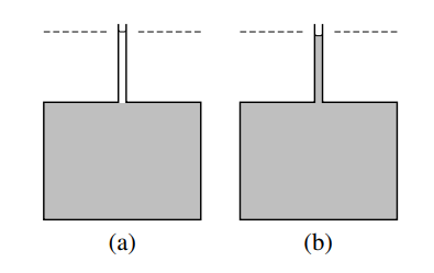
(a) \(40.75 \mathrm{~cm}^3\) (one mole) of methanol is placed in a narrow tube above a much greater volume of a mixture (shaded) of composition \(x_{\mathrm{B}}=0.307\). The dashed line indicates the level of the upper meniscus.
(b) After the two liquid phases have mixed by diffusion, the volume of the mixture has increased by only \(38.8 \mathrm{~cm}^3\).
9.2.1 Partial molar volume
In order to gain insight into the significance of a partial molar quantity as defined by Eq. 9.2.1, let us first apply the concept to the volume of an open single-phase system. Volume has the advantage for our example of being an extensive property that is easily visualized. Let the system be a binary mixture of water (substance A) and methanol (substance B), two liquids that mix in all proportions. The partial molar volume of the methanol, then, is the rate at which the system volume changes with the amount of methanol added to the mixture at constant temperature and pressure: \(V\B=\pd{V}{n\B}{T,p,n\A}\).
At \(25\units{\(\degC\)}\) and \(1\br\), the molar volume of pure water is \(V\mA^* = 18.07\units{cm\(^3\) mol\(^{-1}\)}\) and that of pure methanol is \(V\mB^* = 40.75\units{cm\(^3\) mol\(^{-1}\)}\). If we mix \(100.0\units{cm\(^3\)}\) of water at \(25\units{\(\degC\)}\) with \(100.0\units{cm\(^3\)}\) of methanol at \(25\units{\(\degC\)}\), we find the volume of the resulting mixture at \(25\units{\(\degC\)}\) is not the sum of the separate volumes, \(200.0\units{cm\(^3\)}\), but rather the slightly smaller value \(193.1\units{cm\(^3\)}\). The difference is due to new intermolecular interactions in the mixture compared to the pure liquids.
Let us calculate the mole fraction composition of this mixture:
\[ \begin{equation} n\A = \frac{V\A^*}{V\mA^*} = \frac{100.0\units{cm\(^3\)}}{18.07\units{cm\(^3\) mol\(^{-1}\)}} = 5.53\mol \tag{9.2.2} \end{equation}\]
\[ \begin{equation} n\B = \frac{V\B^*}{V\mB^*} = \frac{100.0\units{cm\(^3\)}}{40.75\units{cm\(^3\) mol\(^{-1}\)}} = 2.45\mol \tag{9.2.3} \end{equation}\]
\[ \begin{equation} x\B = \frac{n\B}{n\A+n\B} = \frac{2.45\mol}{5.53\mol + 2.45\mol} = 0.307 \tag{9.2.4} \end{equation}\]
Now suppose we prepare a large volume of a mixture of this composition \(\left(x_{\mathrm{B}}=0.307\right)\) and add an additional \(40.75 \mathrm{~cm}^3\) (one mole) of pure methanol, as shown in Fig. 9.1(a). If the initial volume of the mixture at \(25^{\circ} \mathrm{C}\) was \(10,000.0 \mathrm{~cm}^3\), we find the volume of the new mixture at the same temperature is \(10,038.8 \mathrm{~cm}^3\), an increase of \(38.8 \mathrm{~cm}^3\) - see Fig. 9.1(b). The amount of methanol added is not infinitesimal, but it is small enough compared to the amount of initial mixture to cause very little change in the mixture composition: \(x_{\mathrm{B}}\)
increases by only \(0.5 \%\). Treating the mixture as an open system, we see that the addition of one mole of methanol to the system at constant \(T, p\), and \(n_{\mathrm{A}}\) causes the system volume to increase by \(38.8 \mathrm{~cm}^3\). To a good approximation, then, the partial molar volume of methanol in the mixture, \(V_{\mathrm{B}}=\left(\partial V / \partial n_{\mathrm{B}}\right)_{T, p, n_{\mathrm{A}}}\), is given by \(\Delta V / \Delta n_{\mathrm{B}}=38.8 \mathrm{~cm}^3 \mathrm{~mol}^{-1}\).
The volume of the mixture to which we add the methanol does not matter as long as it is large. We would have observed practically the same volume increase, \(38.8 \mathrm{~cm}^3\), if we had mixed one mole of pure methanol with \(100,000.0 \mathrm{~cm}^3\) of the mixture instead of only \(10,000.0 \mathrm{~cm}^3\).
Thus, we may interpret the partial molar volume of B as the volume change per amount of B added at constant \(T\) and \(p\) when B is mixed with such a large volume of mixture that the composition is not appreciably affected. We may also interpret the partial molar volume as the volume change per amount when an infinitesimal amount is mixed with a finite volume of mixture.
The partial molar volume of \(\mathrm{B}\) is an intensive property that is a function of the composition of the mixture, as well as of \(T\) and \(p\). The limiting value of \(V_{\mathrm{B}}\) as \(x_{\mathrm{B}}\) approaches 1 (pure B) is \(V_{\mathrm{m}, \mathrm{B}}^*\), the molar volume of pure \(\mathrm{B}\). We can see this by writing \(V=n_{\mathrm{B}} V_{\mathrm{m}, \mathrm{B}}^*\) for pure \(\mathrm{B}\), giving us \(V_{\mathrm{B}}\left(x_{\mathrm{B}}=1\right)=\left(\partial n_{\mathrm{B}} V_{\mathrm{m}, \mathrm{B}}^* / \partial n_{\mathrm{B}}\right)_{T, p, n_{\mathrm{A}}}=V_{\mathrm{m}, \mathrm{B}}^*\).
If the mixture is a binary mixture of \(\mathrm{A}\) and \(\mathrm{B}\), and \(x_{\mathrm{B}}\) is small, we may treat the mixture as a dilute solution of solvent \(\mathrm{A}\) and solute \(\mathrm{B}\). As \(x_{\mathrm{B}}\) approaches 0 in this solution, \(V_{\mathrm{B}}\) approaches a certain limiting value that is the volume increase per amount of B mixed with a large amount of pure A. In the resulting mixture, each solute molecule is surrounded only by solvent molecules. We denote this limiting value of \(V_{\mathrm{B}}\) by \(V_{\mathrm{B}}^{\infty}\), the partial molar volume of solute B at infinite dilution.
It is possible for a partial molar volume to be negative. Magnesium sulfate, in aqueous solutions of molality less than \(0.07 \mathrm{~mol} \mathrm{~kg}^{-1}\), has a negative partial molar volume. Physically, this means that when a small amount of crystalline \(\mathrm{MgSO}_4\) dissolves at constant temperature in water, the liquid phase contracts. This unusual behavior is due to strong attractive water-ion interactions.
9.2.2 The total differential of the volume in an open system
Consider an open single-phase system consisting of a mixture of nonreacting substances. How many independent variables does this system have?
We can prepare the mixture with various amounts of each substance, and we are able to adjust the temperature and pressure to whatever values we wish (within certain limits that prevent the formation of a second phase). Each choice of temperature, pressure, and amounts results in a definite value of every other property, such as volume, density, and mole fraction composition. Thus, an open single-phase system of \(C\) substances has \(2+C\) independent variables. \({ }^3\)
3. C in this kind of system is actually the number of components. The number of components is usually the same as the number of substances, but is less if certain constraints exist, such as reaction equilibrium or a fixed mixture composition. The general meaning of C will be discussed in Sec. 13.
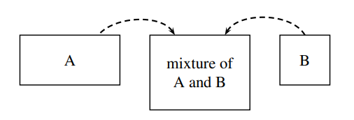
Figure \(\PageIndex{2}\): Mixing of water (A) and methanol (B) in a 2:1 ratio of volumes to form a mixture of increasing volume and constant composition. The system is the mixture.
For a binary mixture \((C=2)\), the number of independent variables is four. We may choose these variables to be \(T, p, n_{\mathrm{A}}\), and \(n_{\mathrm{B}}\), and write the total differential of \(V\) in the general form
\[
\begin{aligned}
\mathrm{d} V= & \left(\frac{\partial V}{\partial T}\right)_{p, n_{\mathrm{A}}, n_{\mathrm{B}}} \mathrm{d} T+\left(\frac{\partial V}{\partial p}\right)_{T, n_{\mathrm{A}}, n_{\mathrm{B}}} \mathrm{d} p \\
& +\left(\frac{\partial V}{\partial n_{\mathrm{A}}}\right)_{T, p, n_{\mathrm{B}}} \mathrm{d} n_{\mathrm{A}}+\left(\frac{\partial V}{\partial n_{\mathrm{B}}}\right)_{T, p, n_{\mathrm{A}}} \mathrm{d} n_{\mathrm{B}}
\end{aligned}
\]
(binary mixture)
We know the first two partial derivatives on the right side are given by \({ }^4\)
4. See Eqs. 7.1.1 and 7.1.2, which are for closed syste
\[
\left(\frac{\partial V}{\partial T}\right)_{p, n_{\mathrm{A}}, n_{\mathrm{B}}}=\alpha V \quad\left(\frac{\partial V}{\partial p}\right)_{T, n_{\mathrm{A}}, n_{\mathrm{B}}}=-\kappa_T V
\]
We identify the last two partial derivatives on the right side of Eq. 9.2.5 as the partial molar volumes \(V_{\mathrm{A}}\) and \(V_{\mathrm{B}}\). Thus, we may write the total differential of \(V\) for this open system in the compact form
\[
\mathrm{d} V=\alpha V \mathrm{~d} T-\kappa_T V \mathrm{~d} p+V_{\mathrm{A}} \mathrm{d} n_{\mathrm{A}}+V_{\mathrm{B}} \mathrm{d} n_{\mathrm{B}}
\]
(binary mixture)
If we compare this equation with the total differential of \(V\) for a one-component closed system, \(\mathrm{d} V=\alpha V \mathrm{~d} T-\kappa_T V \mathrm{~d} p\) (Eq. 7.1.6), we see that an additional term is required for each constituent of the mixture to allow the system to be open and the composition to vary.
When \(T\) and \(p\) are held constant, Eq. 9.2.7 becomes
\[
\mathrm{d} V=V_{\mathrm{A}} \mathrm{d} n_{\mathrm{A}}+V_{\mathrm{B}} \mathrm{d} n_{\mathrm{B}}
\]
(binary mixture, constant \(T\) and \(p\) )
We obtain an important relation between the mixture volume and the partial molar volumes by imagining the following process. Suppose we continuously pour pure water and pure methanol at constant but not necessarily equal volume rates into a stirred, thermostatted container to form a mixture of increasing volume and constant composition, as shown schematically in Fig. 9.2. If this mixture remains at constant \(T\) and \(p\) as it is formed, none of its intensive properties change during the process, and the partial molar volumes \(V_{\mathrm{A}}\) and \(V_{\mathrm{B}}\) remain constant. Under these conditions, we can integrate Eq. 9.2.8 to obtain the additivity
rule for volume: \({ }^5\)
\[
V=V_{\mathrm{A}} n_{\mathrm{A}}+V_{\mathrm{B}} n_{\mathrm{B}}
\]
(binary mixture)
This equation allows us to calculate the mixture volume from the amounts of the constituents and the appropriate partial molar volumes for the particular temperature, pressure, and composition.
For example, given that the partial molar volumes in a water-methanol mixture of composition \(x_{\mathrm{B}}=0.307\) are \(V_{\mathrm{A}}=17.74 \mathrm{~cm}^3 \mathrm{~mol}^{-1}\) and \(V_{\mathrm{B}}=38.76 \mathrm{~cm}^3 \mathrm{~mol}^{-1}\), we calculate the volume of the water-methanol mixture described at the beginning of Sec. 9.2.1 as follows:
\[
\begin{aligned}
V & =\left(17.74 \mathrm{~cm}^3 \mathrm{~mol}^{-1}\right)(5.53 \mathrm{~mol})+\left(38.76 \mathrm{~cm}^3 \mathrm{~mol}^{-1}\right)(2.45 \mathrm{~mol}) \\
& =193.1 \mathrm{~cm}^3
\end{aligned}
\]
We can differentiate Eq. 9.2.9 to obtain a general expression for \(\mathrm{d} V\) under conditions of constant \(T\) and \(p\) :
\[
\mathrm{d} V=V_{\mathrm{A}} \mathrm{d} n_{\mathrm{A}}+V_{\mathrm{B}} \mathrm{d} n_{\mathrm{B}}+n_{\mathrm{A}} \mathrm{d} V_{\mathrm{A}}+n_{\mathrm{B}} \mathrm{d} V_{\mathrm{B}}
\]
But this expression for \(\mathrm{d} V\) is consistent with Eq. 9.2.8 only if the sum of the last two terms on the right is zero:
\[
n_{\mathrm{A}} \mathrm{d} V_{\mathrm{A}}+n_{\mathrm{B}} \mathrm{d} V_{\mathrm{B}}=0
\]
(binary mixture, constant \(T\) and \(p\) )
Equation 9.2.12 is the Gibbs-Duhem equation for a binary mixture, applied to partial molar volumes. (Section 9.2.4 will give a general version of this equation.) Dividing both sides of the equation by \(n_{\mathrm{A}}+n_{\mathrm{B}}\) gives the equivalent form
\[
x_{\mathrm{A}} \mathrm{d} V_{\mathrm{A}}+x_{\mathrm{B}} \mathrm{d} V_{\mathrm{B}}=0
\]
(binary mixture, constant \(T\) and \(p\) )
Equation 9.2.12 shows that changes in the values of \(V_{\mathrm{A}}\) and \(V_{\mathrm{B}}\) are related when the composition changes at constant \(T\) and \(p\). If we rearrange the equation to the form
\[
\mathrm{d} V_{\mathrm{A}}=-\frac{n_{\mathrm{B}}}{n_{\mathrm{A}}} \mathrm{d} V_{\mathrm{B}}
\]
(binary mixture, constant \(T\) and \(p\) )
we see that a composition change that increases \(V_{\mathrm{B}}\) (so that \(\mathrm{d} V_{\mathrm{B}}\) is positive) must make \(V_{\mathrm{A}}\) decrease.
9.2.3 Evaluation of partial molar volumes in binary mixtures
The partial molar volumes \(V_{\mathrm{A}}\) and \(V_{\mathrm{B}}\) in a binary mixture can be evaluated by the method of intercepts. To use this method, we plot experimental values of the quantity \(V / n\) (where \(n\) is \(n_{\mathrm{A}}+n_{\mathrm{B}}\) ) versus the mole fraction \(x_{\mathrm{B}} . V / n\) is called the mean molar volume.
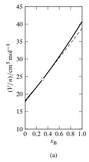
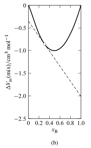
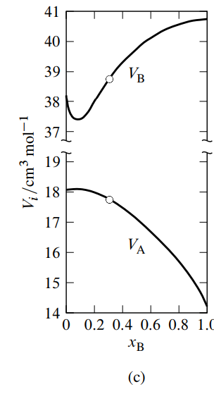
Figure \(\PageIndex{3}\): Figure 9.3 Mixtures of water (A) and methanol (B) at \(25^{\circ} \mathrm{C}\) and 1 bar. \({ }^a\)
- Mean molar volume as a function of \(x_{\mathrm{B}}\). The dashed line is the tangent to the curve at \(x_{\mathrm{B}}=0.307\).
- Molar volume of mixing as a function of \(x_{\mathrm{B}}\). The dashed line is the tangent to the curve at \(x_{\mathrm{B}}=0.307\).
- Partial molar volumes as functions of \(x_{\mathrm{B}}\). The points at \(x_{\mathrm{B}}=0.307\) (open circles) are obtained from the intercepts of the dashed line in either (a) or (b).
\({ }^a\) Based on data in Ref. [12].
See Fig. 9.3(a) for an example. In this figure, the tangent to the curve drawn at the point on the curve at the composition of interest (the composition used as an illustration in Sec. 9.2.1) intercepts the vertical line where \(x\B\) equals \(0\) at \(V/n = V\A = 17.7\units{cm\(^3\) mol\(^{-1}\)}\), and intercepts the vertical line where \(x\B\) equals \(1\) at \(V/n = V\B = 38.8\units{cm\(^3\) mol\(^{-1}\)}\).
To derive this property of a tangent line for the plot of \(V/n\) versus \(x\B\), we use Eq. 9.2.9 to write \begin{equation} \begin{split} (V/n) & = \frac{ V\A n\A + V\B n\B}{n} = V\A x\A + V\B x\B \cr & =V\A(1-x\B) + V\B x\B = (V\B - V\A)x\B + V\A \end{split} \tag{9.2.15} \end{equation}
\({ }^5\) The equation is an example of the result of applying Euler's theorem on homogeneous functions to \(V\) treated as a function of \(n_{\mathrm{A}}\) and \(n_{\mathrm{B}}\).
When we differentiate this expression for \(V/n\) with respect to \(x\B\), keeping in mind that \(V\A\) and \(V\B\) are functions of \(x\B\), we obtain \begin{equation} \begin{split} \frac{\dif (V/n)}{\dx\B} & = \frac{\dif[(V\B - V\A)x\B + V\A]}{\dx\B}\cr & = V\B - V\A + \left( \frac{\dif V\B}{\dx\B} - \frac{\dif V\A}{\dx\B} \right)x\B + \frac{\dif V\A}{\dx\B} \cr & = V\B - V\A + \left(\frac{\dif V\A}{\dx\B}\right)(1-x\B) + \left(\frac{\dif V\B}{\dx\B}\right)x\B \cr & = V\B - V\A + \left(\frac{\dif V\A}{\dx\B}\right)x\A + \left(\frac{\dif V\B}{\dx\B}\right)x\B \end{split} \tag{9.2.16} \end{equation}
The differentials \(\dif V\A\) and \(\dif V\B\) are related to one another by the Gibbs–Duhem equation (Eq. 9.2.13): \(x\A\dif V\A + x\B\dif V\B = 0\). We divide both sides of this equation by \(\dx\B\) to obtain \begin{equation} \left(\frac{\dif V\A}{\dx\B}\right)x\A + \left(\frac{\dif V\B}{\dx\B}\right)x\B = 0 \tag{9.2.17} \end{equation} and substitute in Eq. 9.2.16 to obtain \begin{equation} \frac{\dif(V/n)}{\dx\B} = V\B - V\A \tag{9.2.18} \end{equation}
Let the partial molar volumes of the constituents of a binary mixture of arbitrary composition \(x'\B\) be \(V'\A\) and \(V'\B\). Equation 9.2.15 shows that the value of \(V/n\) at the point on the curve of \(V/n\) versus \(x\B\) where the composition is \(x'\B\) is \((V'\B-V'\A)x'\B+V'\A\). Equation 9.2.18 shows that the tangent to the curve at this point has a slope of \(V'\B - V'\A\). The equation of the line that passes through this point and has this slope, and thus is the tangent to the curve at this point, is \(y=(V'\B - V'\A)x\B + V'\A\), where \(y\) is the vertical ordinate on the plot of \((V/n)\) versus \(x\B\). The line has intercepts \(y{=}V'\A\) at \(x\B{=}0\) and \(y{=}V'\B\) at \(x\B{=}1\).
A variant of the method of intercepts is to plot the molar integral volume of mixing given by \begin{equation} \Del V\m\mix = \frac{\Del V\mix}{n} = \frac{V-n\A V\mA^*-n\B V\mB^*}{n} \tag{9.2.19} \end{equation} versus \(x\B\), as illustrated in Fig. 9.3(b). \(\Del V\mix\) is the integral volume of mixing—the volume change at constant \(T\) and \(p\) when solvent and solute are mixed to form a mixture of volume \(V\) and total amount \(n\) (see Sec. 11.1.1). The tangent to the curve at the composition of interest has intercepts \(V\A-V\mA^*\) at \(x\B{=}0\) and \(V\B-V\mB^*\) at \(x\B{=}1\).
To see this, we write \begin{equation} \begin{split} \Del V\m\mix & = (V/n) - x\A V\mA^* - x\B V\mB^* \cr & = (V/n) - (1- x\B)V\mA^* - x\B V\mB^* \end{split} \tag{9.2.20} \end{equation} We make the substitution \((V/n)=(V\B-V\A)x\B+V\A\) from Eq. 9.2.15 and rearrange: \begin{equation} \Del V\m\mix = \left[\left( V\B-V\mB^* \right) - \left( V\A-V\mA^* \right) \right]x\B + \left( V\A-V\mA^* \right) \tag{9.2.21} \end{equation} Differentiation with respect to \(x\B\) yields \begin{equation} \begin{split} \frac{\dif \Del V\m\mix}{\dx\B} & = \left( V\B-V\mB^* \right) - \left( V\A-V\mA^* \right) + \left( \frac{\dif V\B}{\dx\B}-\frac{\dif V\A}{\dx\B} \right)x\B + \frac{\dif V\A}{\dx\B} \cr & = \left( V\B-V\mB^* \right) - \left( V\A-V\mA^* \right) + \left(\frac{\dif V\A}{\dx\B}\right)(1-x\B) + \left(\frac{\dif V\B}{\dx\B}\right)x\B \cr & = \left( V\B-V\mB^* \right) - \left( V\A-V\mA^* \right) + \left(\frac{\dif V\A}{\dx\B}\right)x\A + \left(\frac{\dif V\B}{\dx\B}\right)x\B \end{split} \tag{9.2.22} \end{equation} With a substitution from Eq. 9.2.17, this becomes \begin{equation} \frac{\dif \Del V\m\mix}{\dx\B} = \left( V\B-V\mB^* \right) - \left( V\A-V\mA^* \right) \tag{9.2.23} \end{equation} Equations 9.2.21 and 9.2.23 are analogous to Eqs. 9.2.15 and 9.2.18, with \(V/n\) replaced by \(\Del V\m\mix\), \(V\A\) by \((V\A-V\mA^*)\), and \(V\B\) by \((V\B-V\mB^*)\). Using the same reasoning as for a plot of \(V/n\) versus \(x\B\), we find the intercepts of the tangent to a point on the curve of \(\Del V\m\mix\) versus \(x\B\) are at \(V\A-V\mA^*\) and \(V\B-V\mB^*\).
Figure 9.3 shows smoothed experimental data for water–methanol mixtures plotted in both kinds of graphs, and the resulting partial molar volumes as functions of composition. Note in Fig. 9.3(c) how the \(V\A\) curve mirrors the \(V\B\) curve as \(x\B\) varies, as predicted by the Gibbs–Duhem equation. The minimum in \(V\B\) at \(x\B {\approx} 0.09\) is mirrored by a maximum in \(V\A\) in agreement with Eq. 9.2.14; the maximum is much attenuated because \(n\B/n\A\) is much less than unity.
Macroscopic measurements are unable to provide unambiguous information about molecular structure. Nevertheless, it is interesting to speculate on the implications of the minimum observed for the partial molar volume of methanol. One interpretation is that in a mostly aqueous environment, there is association of methanol molecules, perhaps involving the formation of dimers.
9.2.4 General relations
The discussion above of partial molar volumes used the notation \(V\mA^*\) and \(V\mB^*\) for the molar volumes of pure A and B. The partial molar volume of a pure substance is the same as the molar volume, so we can simplify the notation by using \(V\A^*\) and \(V\B^*\) instead. Hereafter, this e-book will denote molar quantities of pure substances by such symbols as \(V\A^*\), \(H\B^*\), and \(S_i^*\).
The relations derived above for the volume of a binary mixture may be generalized for any extensive property \(X\) of a mixture of any number of constituents. The partial molar quantity of species \(i\), defined by \begin{equation} X_i \defn \Pd{X}{n_i}{T,p,n_{j\ne i}} \tag{9.2.24} \end{equation} is an intensive property that depends on \(T\), \(p\), and the composition of the mixture. The additivity rule for property \(X\) is \begin{gather} \s{ X = \sum_i n_i X_i } \tag{9.2.25} \cond{(mixture)} \end{gather} and the Gibbs–Duhem equation applied to \(X\) can be written in the equivalent forms \begin{gather} \s{ \sum_i n_i \dif X_i = 0 } \tag{9.2.26} \cond{(constant \(T\) and \(p\))} \end{gather} and \begin{gather} \s{ \sum_i x_i \dif X_i = 0 } \tag{9.2.27} \cond{(constant \(T\) and \(p\))} \end{gather} These relations can be applied to a mixture in which each species \(i\) is a nonelectrolyte substance, an electrolyte substance that is dissociated into ions, or an individual ionic species. In Eq. 9.2.27, the mole fraction \(x_i\) must be based on the different species considered to be present in the mixture. For example, an aqueous solution of NaCl could be treated as a mixture of components A=H\(_2\)O and B=NaCl, with \(x\B\) equal to \(n\B/(n\A+n\B)\); or the constituents could be taken as H\(_2\)O, Na\(^+\), and Cl\(^-\), in which case the mole fraction of Na\(^+\) would be \(x_+=n_+/(n\A+n_++n_-)\).
A general method to evaluate the partial molar quantities \(X\A\) and \(X\B\) in a binary mixture is based on the variant of the method of intercepts described in Sec. 9.2.3. The molar mixing quantity \(\Del X\mix/n\) is plotted versus \(x\B\), where \(\Del X\mix\) is \((X{-}n\A X\A^*{-}n\B X\B^*)\). On this plot, the tangent to the curve at the composition of interest has intercepts equal to \(X\A{-}X\A^*\) at \(x\B{=}0\) and \(X\B{-}X\B^*\) at \(x\B{=}1\).
We can obtain experimental values of such partial molar quantities of an uncharged species as \(V_i\), \(C_{p,i}\), and \(S_i\). It is not possible, however, to evaluate the partial molar quantities \(U_i\), \(H_i\), \(A_i\), and \(G_i\) because these quantities involve the internal energy brought into the system by the species, and we cannot evaluate the absolute value of internal energy (Sec. 2.6.2). For example, while we can evaluate the difference \(H_i-H_i^*\) from calorimetric measurements of enthalpies of mixing, we cannot evaluate the partial molar enthalpy \(H_i\) itself. We can, however, include such quantities as \(H_i\) in useful theoretical relations.
A partial molar quantity of a charged species is something else we cannot evaluate. It is possible, however, to obtain values relative to a reference ion. Consider an aqueous solution of a fully-dissociated electrolyte solute with the formula \(\tx{M}_{\nu_+}\tx{X}_{\nu_-}\), where \(\nu_+\) and \(\nu_-\) are the numbers of cations and anions per solute formula unit. The partial molar volume \(V\B\) of the solute, which can be determined experimentally, is related to the (unmeasurable) partial molar volumes \(V_+\) and \(V_-\) of the constituent ions by \begin{equation} V\B = \nu_+ V_+ + \nu_- V_- \tag{9.2.28} \end{equation} For aqueous solutions, the usual reference ion is H\(^+\), and the partial molar volume of this ion at infinite dilution is arbitrarily set equal to zero: \(V\subs{H\(^+\)}^{\infty}=0\).
For example, given the value (at \(298.15\K\) and \(1\br\)) of the partial molar volume at infinite dilution of aqueous hydrogen chloride \begin{equation} V\subs{HCl}^{\infty}=17.82\units{cm\(^3\) mol\(^{-1}\)} \tag{9.2.29} \end{equation} we can find the so-called “conventional” partial molar volume of Cl\(^-\) ion: \begin{equation} V\subs{Cl\(^-\)}^{\infty}=V\subs{HCl}^{\infty}-V\subs{H\(^+\)}^{\infty}=17.82\units{cm\(^3\) mol\(^{-1}\)} \tag{9.2.30} \end{equation} Going one step further, the measured value \(V\subs{NaCl}^{\infty}=16.61\units{cm\(^3\) mol\(^{-1}\)}\) gives, for Na\(^+\) ion, the conventional value \begin{equation} V\subs{Na\(^+\)}^{\infty}=V\subs{NaCl}^{\infty}-V\subs{Cl\(^-\)}^{\infty} = (16.61-17.82)\units{cm\(^3\) mol\(^{-1}\)} = -1.21\units{cm\(^3\) mol\(^{-1}\)} \tag{9.2.31} \end{equation}
9.2.5 Partial specific quantities
A partial specific quantity of a substance is the partial molar quantity divided by the molar mass, and has dimensions of volume divided by mass. For example, the partial specific volume \(v\B\) of solute B in a binary solution is given by \begin{equation} v\B=\frac{V\B}{M\B} = \bPd{V}{m(\tx{B})}{T,p,m(\tx{A})} \tag{9.2.32} \end{equation} where \(m(\tx{A})\) and \(m(\tx{B})\) are the masses of solvent and solute.
Although this e-book makes little use of specific quantities and partial specific quantities, in some applications they have an advantage over molar quantities and partial molar quantities because they can be evaluated without knowledge of the molar mass. For instance, the value of a solute’s partial specific volume is used to determine its molar mass by the method of sedimentation equilibrium (Sec. 9.8.2).
The general relations in Sec. 9.2.4 involving partial molar quantities may be turned into relations involving partial specific quantities by replacing amounts by masses, mole fractions by mass fractions, and partial molar quantities by partial specific quantities. Using volume as an example, we can write an additivity relation \(V=\sum_i m(i)v_i\), and Gibbs–Duhem relations \(\sum_i m(i)\dif v_i=0\) and \(\sum_i w_i\dif v_i=0\). For a binary mixture of A and B, we can plot the specific volume \(v\) versus the mass fraction \(w\B\); then the tangent to the curve at a given composition has intercepts equal to \(v\A\) at \(w\B{=}0\) and \(v\B\) at \(w\B{=}1\). A variant of this plot is \(\left(v-w\A v\A^*-w\B v\B^*\right)\) versus \(w\B\); the intercepts are then equal to \(v\A-v\A^*\) and \(v\B-v\B^*\).
9.2.6 The chemical potential of a species in a mixture
Just as the molar Gibbs energy of a pure substance is called the chemical potential and given the special symbol \(\mu\), the partial molar Gibbs energy \(G_i\) of species \(i\) in a mixture is called the chemical potential of species \(i\), defined by \begin{gather} \s{ \mu_i \defn \Pd{G}{n_i}{T,p,n_{j \ne i}} } \tag{9.2.33} \cond{(mixture)} \end{gather} If there are work coordinates for nonexpansion work, the partial derivative is taken at constant values of these coordinates.
The chemical potential of a species in a phase plays a crucial role in equilibrium problems, because it is a measure of the escaping tendency of the species from the phase. Although we cannot determine the absolute value of \(\mu_i\) for a given state of the system, we are usually able to evaluate the difference between the value in this state and the value in a defined reference state.
In an open single-phase system containing a mixture of \(s\) different nonreacting species, we may in principle independently vary \(T\), \(p\), and the amount of each species. This is a total of \(2 + s\) independent variables. The total differential of the Gibbs energy of this system is given by Eq. 5.5.9, often called the Gibbs fundamental equation: \begin{gather} \s{ \dif G = -S\dif T + V\difp + \sum_{i=1}^{s} \mu_i \dif n_i } \tag{9.2.34} \cond{(mixture)} \end{gather}
Consider the special case of a mixture containing charged species, for example an aqueous solution of the electrolyte KCl. We could consider the constituents to be either the substances H\(_2\)O and KCl, or else H\(_2\)O and the species K\(^+\) and Cl\(^-\). Any mixture we can prepare in the laboratory must remain electrically neutral, or virtually so. Thus, while we are able to independently vary the amounts of H\(_2\)O and KCl, we cannot in practice independently vary the amounts of K\(^+\) and Cl\(^-\) in the mixture. The chemical potential of the K\(^+\) ion is defined as the rate at which the Gibbs energy changes with the amount of K\(^+\) added at constant \(T\) and \(p\) while the amount of Cl\(^-\) is kept constant. This is a hypothetical process in which the net charge of the mixture increases. The chemical potential of a ion is therefore a valid but purely theoretical concept. Let A stand for H\(_2\)O, B for KCl, \(+\) for K\(^+\), and \(-\) for Cl\(^-\). Then it is theoretically valid to write the total differential of \(G\) for the KCl solution either as \begin{equation} \dif G = -S\dif T + V\difp + \mu\A\dif n\A + \mu\B\dif n\B \tag{9.2.35} \end{equation} or as \begin{equation} \dif G = -S\dif T + V\difp + \mu\A\dif n\A + \mu_+\dif n_+ + \mu_-\dif n_- \tag{9.2.36} \end{equation}
9.2.7 Equilibrium conditions in a multiphase, multicomponent system
This section extends the derivation described in Sec. 8.1.2, which was for equilibrium conditions in a multiphase system containing a single substance, to a more general kind of system: one with two or more homogeneous phases containing mixtures of nonreacting species. The derivation assumes there are no internal partitions that could prevent transfer of species and energy between the phases, and that effects of gravity and other external force fields are negligible.
The system consists of a reference phase, \(\pha'\), and other phases labeled by \(\pha{\ne}\pha'\). Species are labeled by subscript \(i\). Following the procedure of Sec. 8.1.1, we write for the total differential of the internal energy \begin{equation} \begin{split} \dif U & = \dif U\aphp + \sum_{\pha\ne\pha'}\dif U\aph \cr & = T\aphp\dif S\aphp - p\aphp\dif V\aphp + \sum_i\mu_i\aphp\dif n_i\aphp \cr & \quad + \sum_{\pha\ne\pha'}\left(T\aph\dif S\aph - p\aph\dif V\aph + \sum_i\mu_i\aph\dif n_i\aph\right) \end{split} \tag{9.2.37} \end{equation} The conditions of isolation are \begin{equation} \dif U = 0 \qquad \tx{(constant internal energy)} \tag{9.2.38} \end{equation} \begin{equation} \dif V\aphp + \sum_{\pha\ne\pha'}\dif V\aph = 0 \qquad \tx{(no expansion work)} \tag{9.2.39} \end{equation} \begin{equation} \begin{split} &\tx{For each species \(i\):} \cr &\dif n_i\aphp + \sum_{\pha\ne\pha'}\dif n_i\aph = 0 \qquad \tx{(closed system)} \end{split} \tag{9.2.40} \end{equation} We use these relations to substitute for \(\dif U\), \(\dif V\aphp\), and \(\dif n_i\aphp\) in Eq. 9.2.37. After making the further substitution \(\dif S\aphp = \dif S - \sum_{\pha\ne\pha'}\dif S\aph\) and solving for \(\dif S\), we obtain \begin{equation} \dif S = \sum_{\pha\ne\pha'}\frac{T\aphp-T\aph}{T\aphp}\dif S\aph - \sum_{\pha\ne\pha'}\frac{p\aphp-p\aph}{T\aphp}\dif V\aph + \sum_i\sum_{\pha\ne\pha'}\frac{\mu_i\aphp-\mu_i\aph}{T\aphp}\dif n_i\aph \tag{9.2.41} \end{equation} This equation is like Eq. 8.1.6 with provision for more than one species.
In the equilibrium state of the isolated system, \(S\) has the maximum possible value, \(\dif S\) is equal to zero for an infinitesimal change of any of the independent variables, and the coefficient of each term on the right side of Eq. 9.2.41 is zero. We find that in this state each phase has the same temperature and the same pressure, and for each species the chemical potential is the same in each phase.
Suppose the system contains a species \(i'\) that is effectively excluded from a particular phase, \(\pha''\). For instance, sucrose molecules dissolved in an aqueous phase are not accommodated in the crystal structure of an ice phase, and a nonpolar substance may be essentially insoluble in an aqueous phase. We can treat this kind of situation by setting \(\dif n^{\pha''}_{i'}\) equal to zero. Consequently there is no equilibrium condition involving the chemical potential of this species in phase \(\pha''\).
To summarize these conclusions: In an equilibrium state of a multiphase, multicomponent system without internal partitions, the temperature and pressure are uniform throughout the system, and each species has a uniform chemical potential except in phases where it is excluded.
This statement regarding the uniform chemical potential of a species applies to both a substance and an ion, as the following argument explains. The derivation in this section begins with Eq. 9.2.37, an expression for the total differential of \(U\). Because it is a total differential, the expression requires the amount \(n_i\) of each species \(i\) in each phase to be an independent variable. Suppose one of the phases is the aqueous solution of KCl used as an example at the end of the preceding section. In principle (but not in practice), the amounts of the species H\(_2\)O, K\(^+\), and Cl\(^-\) can be varied independently, so that it is valid to include these three species in the sums over \(i\) in Eq. 9.2.37. The derivation then leads to the conclusion that K\(^+\) has the same chemical potential in phases that are in transfer equilibrium with respect to K\(^+\), and likewise for Cl\(^-\). This kind of situation arises when we consider a Donnan membrane equilibrium (Sec. 12.7.3) in which transfer equilibrium of ions exists between solutions of electrolytes separated by a semipermeable membrane.
9.2.8 Relations involving partial molar quantities
Here we derive several useful relations involving partial molar quantities in a single-phase system that is a mixture. The independent variables are \(T\), \(p\), and the amount \(n_i\) of each constituent species \(i\).
From Eqs. 9.2.26 and 9.2.27, the Gibbs–Duhem equation applied to the chemical potentials can be written in the equivalent forms \begin{gather} \s{ \sum_i n_i \dif\mu_i = 0 } \tag{9.2.42} \cond{(constant \(T\) and \(p\))} \end{gather} and \begin{gather} \s{ \sum_i x_i \dif\mu_i = 0 } \tag{9.2.43} \cond{(constant \(T\) and \(p\))} \end{gather} These equations show that the chemical potentials of different species cannot be varied independently at constant \(T\) and \(p\).
A more general version of the Gibbs–Duhem equation, without the restriction of constant \(T\) and \(p\), is \begin{equation} S\dif T - V\difp + \sum_i n_i \dif\mu_i = 0 \tag{9.2.44} \end{equation} This version is derived by comparing the expression for \(\dif G\) given by Eq. 9.2.34 with the differential \(\dif G {=} \sum_i \mu_i\dif n_i {+} \sum_i n_i\dif\mu_i\) obtained from the additivity rule \(G {=} \sum_i \mu_i n_i\).
The Gibbs energy is defined by \(G=H-TS\). Taking the partial derivatives of both sides of this equation with respect to \(n_i\) at constant \(T\), \(p\), and \(n_{j \ne i}\) gives us \begin{equation} \Pd{G}{n_i}{T,p,n_{j \ne i}} = \Pd{H}{n_i}{T,p,n_{j \ne i}} - T\Pd{S}{n_i}{T,p,n_{j \ne i}} \tag{9.2.45} \end{equation} We recognize each partial derivative as a partial molar quantity and rewrite the equation as \begin{equation} \mu_i = H_i -TS_i \tag{9.2.46} \end{equation} This is analogous to the relation \(\mu=G/n=H\m-TS\m\) for a pure substance.
From the total differential of the Gibbs energy, \(\dif G = -S\dif T + V\difp + \sum_i \mu_i\dif n_i\) (Eq. 9.2.34), we obtain the following reciprocity relations: \begin{equation} \Pd{\mu_i}{T}{p,\allni} = -\Pd{S}{n_i}{T,p,n_{j \ne i}} \qquad \Pd{\mu_i}{p}{T,\allni} = \Pd{V}{n_i}{T,p,n_{j \ne i}} \tag{9.2.47} \end{equation} The symbol \(\allni\) stands for the set of amounts of all species, and subscript \(\allni\) on a partial derivative means the amount of each species is constant—that is, the derivative is taken at constant composition of a closed system. Again we recognize partial derivatives as partial molar quantities and rewrite these relations as follows: \begin{equation} \Pd{\mu_i}{T}{p,\allni} = -S_i \tag{9.2.48} \end{equation} \begin{equation} \Pd{\mu_i}{p}{T,\allni} = V_i \tag{9.2.49} \end{equation} These equations are the equivalent for a mixture of the relations \(\pd{\mu}{T}{p} = -S\m\) and \(\pd{\mu}{p}{T} = V\m\) for a pure phase (Eqs. 7.8.3 and 7.8.4).
Taking the partial derivatives of both sides of \(U=H-pV\) with respect to \(n_i\) at constant \(T\), \(p\), and \(n_{j \ne i}\) gives \begin{equation} U_i = H_i - pV_i \tag{9.2.50} \end{equation}
Finally, we can obtain a formula for \(C_{p,i}\), the partial molar heat capacity at constant pressure of species \(i\), by writing the total differential of \(H\) in the form \begin{equation} \begin{split} \dif H & = \Pd{H}{T}{p,\allni}\dif T + \Pd{H}{p}{T,\allni}\difp + \sum_i \Pd{H}{n_i}{T,p,n_{j \ne i}}\dif n_i \cr & = C_p\dif T + \Pd{H}{p}{T,\allni}\difp + \sum_i H_i\dif n_i \end{split} \tag{9.2.51} \end{equation} from which we have the reciprocity relation \(\pd{C_p}{n_i}{T,p,n_{j \ne i}} = \pd{H_i}{T}{p,\allni}\), or \begin{equation} C_{p,i} = \Pd{H_i}{T}{p,\allni} \tag{9.2.52} \end{equation}