
7.3: Thermal Properties
- Page ID
- 20428

\( \newcommand{\vecs}[1]{\overset { \scriptstyle \rightharpoonup} {\mathbf{#1}} } \)
\( \newcommand{\vecd}[1]{\overset{-\!-\!\rightharpoonup}{\vphantom{a}\smash {#1}}} \)
\( \newcommand{\id}{\mathrm{id}}\) \( \newcommand{\Span}{\mathrm{span}}\)
( \newcommand{\kernel}{\mathrm{null}\,}\) \( \newcommand{\range}{\mathrm{range}\,}\)
\( \newcommand{\RealPart}{\mathrm{Re}}\) \( \newcommand{\ImaginaryPart}{\mathrm{Im}}\)
\( \newcommand{\Argument}{\mathrm{Arg}}\) \( \newcommand{\norm}[1]{\| #1 \|}\)
\( \newcommand{\inner}[2]{\langle #1, #2 \rangle}\)
\( \newcommand{\Span}{\mathrm{span}}\)
\( \newcommand{\id}{\mathrm{id}}\)
\( \newcommand{\Span}{\mathrm{span}}\)
\( \newcommand{\kernel}{\mathrm{null}\,}\)
\( \newcommand{\range}{\mathrm{range}\,}\)
\( \newcommand{\RealPart}{\mathrm{Re}}\)
\( \newcommand{\ImaginaryPart}{\mathrm{Im}}\)
\( \newcommand{\Argument}{\mathrm{Arg}}\)
\( \newcommand{\norm}[1]{\| #1 \|}\)
\( \newcommand{\inner}[2]{\langle #1, #2 \rangle}\)
\( \newcommand{\Span}{\mathrm{span}}\) \( \newcommand{\AA}{\unicode[.8,0]{x212B}}\)
\( \newcommand{\vectorA}[1]{\vec{#1}} % arrow\)
\( \newcommand{\vectorAt}[1]{\vec{\text{#1}}} % arrow\)
\( \newcommand{\vectorB}[1]{\overset { \scriptstyle \rightharpoonup} {\mathbf{#1}} } \)
\( \newcommand{\vectorC}[1]{\textbf{#1}} \)
\( \newcommand{\vectorD}[1]{\overrightarrow{#1}} \)
\( \newcommand{\vectorDt}[1]{\overrightarrow{\text{#1}}} \)
\( \newcommand{\vectE}[1]{\overset{-\!-\!\rightharpoonup}{\vphantom{a}\smash{\mathbf {#1}}}} \)
\( \newcommand{\vecs}[1]{\overset { \scriptstyle \rightharpoonup} {\mathbf{#1}} } \)
\( \newcommand{\vecd}[1]{\overset{-\!-\!\rightharpoonup}{\vphantom{a}\smash {#1}}} \)
\(\newcommand{\avec}{\mathbf a}\) \(\newcommand{\bvec}{\mathbf b}\) \(\newcommand{\cvec}{\mathbf c}\) \(\newcommand{\dvec}{\mathbf d}\) \(\newcommand{\dtil}{\widetilde{\mathbf d}}\) \(\newcommand{\evec}{\mathbf e}\) \(\newcommand{\fvec}{\mathbf f}\) \(\newcommand{\nvec}{\mathbf n}\) \(\newcommand{\pvec}{\mathbf p}\) \(\newcommand{\qvec}{\mathbf q}\) \(\newcommand{\svec}{\mathbf s}\) \(\newcommand{\tvec}{\mathbf t}\) \(\newcommand{\uvec}{\mathbf u}\) \(\newcommand{\vvec}{\mathbf v}\) \(\newcommand{\wvec}{\mathbf w}\) \(\newcommand{\xvec}{\mathbf x}\) \(\newcommand{\yvec}{\mathbf y}\) \(\newcommand{\zvec}{\mathbf z}\) \(\newcommand{\rvec}{\mathbf r}\) \(\newcommand{\mvec}{\mathbf m}\) \(\newcommand{\zerovec}{\mathbf 0}\) \(\newcommand{\onevec}{\mathbf 1}\) \(\newcommand{\real}{\mathbb R}\) \(\newcommand{\twovec}[2]{\left[\begin{array}{r}#1 \\ #2 \end{array}\right]}\) \(\newcommand{\ctwovec}[2]{\left[\begin{array}{c}#1 \\ #2 \end{array}\right]}\) \(\newcommand{\threevec}[3]{\left[\begin{array}{r}#1 \\ #2 \\ #3 \end{array}\right]}\) \(\newcommand{\cthreevec}[3]{\left[\begin{array}{c}#1 \\ #2 \\ #3 \end{array}\right]}\) \(\newcommand{\fourvec}[4]{\left[\begin{array}{r}#1 \\ #2 \\ #3 \\ #4 \end{array}\right]}\) \(\newcommand{\cfourvec}[4]{\left[\begin{array}{c}#1 \\ #2 \\ #3 \\ #4 \end{array}\right]}\) \(\newcommand{\fivevec}[5]{\left[\begin{array}{r}#1 \\ #2 \\ #3 \\ #4 \\ #5 \\ \end{array}\right]}\) \(\newcommand{\cfivevec}[5]{\left[\begin{array}{c}#1 \\ #2 \\ #3 \\ #4 \\ #5 \\ \end{array}\right]}\) \(\newcommand{\mattwo}[4]{\left[\begin{array}{rr}#1 \amp #2 \\ #3 \amp #4 \\ \end{array}\right]}\) \(\newcommand{\laspan}[1]{\text{Span}\{#1\}}\) \(\newcommand{\bcal}{\cal B}\) \(\newcommand{\ccal}{\cal C}\) \(\newcommand{\scal}{\cal S}\) \(\newcommand{\wcal}{\cal W}\) \(\newcommand{\ecal}{\cal E}\) \(\newcommand{\coords}[2]{\left\{#1\right\}_{#2}}\) \(\newcommand{\gray}[1]{\color{gray}{#1}}\) \(\newcommand{\lgray}[1]{\color{lightgray}{#1}}\) \(\newcommand{\rank}{\operatorname{rank}}\) \(\newcommand{\row}{\text{Row}}\) \(\newcommand{\col}{\text{Col}}\) \(\renewcommand{\row}{\text{Row}}\) \(\newcommand{\nul}{\text{Nul}}\) \(\newcommand{\var}{\text{Var}}\) \(\newcommand{\corr}{\text{corr}}\) \(\newcommand{\len}[1]{\left|#1\right|}\) \(\newcommand{\bbar}{\overline{\bvec}}\) \(\newcommand{\bhat}{\widehat{\bvec}}\) \(\newcommand{\bperp}{\bvec^\perp}\) \(\newcommand{\xhat}{\widehat{\xvec}}\) \(\newcommand{\vhat}{\widehat{\vvec}}\) \(\newcommand{\uhat}{\widehat{\uvec}}\) \(\newcommand{\what}{\widehat{\wvec}}\) \(\newcommand{\Sighat}{\widehat{\Sigma}}\) \(\newcommand{\lt}{<}\) \(\newcommand{\gt}{>}\) \(\newcommand{\amp}{&}\) \(\definecolor{fillinmathshade}{gray}{0.9}\)For convenience in derivations to follow, expressions from Chap. 5 are repeated here that apply to processes in a closed system in the absence of nonexpansion work (i.e., đ \(w^{\prime}=0\) ). For a process at constant volume we have \(^{3}\)
\[
\mathrm{d} U=\mathrm{d} q \quad C_{V}=\left(\frac{\partial U}{\partial T}\right)_{V}
\]
and for a process at constant pressure we have \({ }^{4}\)
\[
\mathrm{d} H=\mathrm{d} q \quad C_{p}=\left(\frac{\partial H}{\partial T}\right)_{p}
\]
A closed system of one component in a single phase has only two independent variables. In such a system, the partial derivatives above are complete and unambiguous definitions of \(C_{V}\) and \(C_{p}\) because they are expressed with two independent variables- \(T\) and \(V\) for \(C_{V}\), and \(T\) and \(p\) for \(C_{p}\). As mentioned on page 146, additional conditions would have to be specified to define \(C_{V}\) for a more complicated system; the same is true for \(C_{p}\).
For a closed system of an ideal gas we have 5
\[
C_{V}=\frac{\mathrm{d} U}{\mathrm{~d} T} \quad C_{p}=\frac{\mathrm{d} H}{\mathrm{~d} T}
\]
7.3.1 The relation between \(C_{V, \mathrm{~m}}\) and \(C_{p, \mathrm{~m}}\)
The value of \(C_{p, \mathrm{~m}}\) for a substance is greater than \(C_{V, \mathrm{~m}}\). The derivation is simple in the case of a fixed amount of an ideal gas. Using substitutions from Eq. 7.3.3, we write
\[
C_{p}-C_{V}=\frac{\mathrm{d} H}{\mathrm{~d} T}-\frac{\mathrm{d} U}{\mathrm{~d} T}=\frac{\mathrm{d}(H-U)}{\mathrm{d} T}=\frac{\mathrm{d}(p V)}{\mathrm{d} T}=n R
\]
Division by \(n\) to obtain molar quantities and rearrangement then gives
\[
C_{p, \mathrm{~m}}=C_{V, \mathrm{~m}}+R
\]
For any phase in general, we proceed as follows. First we write
\[
C_{p}=\left(\frac{\partial H}{\partial T}\right)_{p}=\left[\frac{\partial(U+p V)}{\partial T}\right]_{p}=\left(\frac{\partial U}{\partial T}\right)_{p}+p\left(\frac{\partial V}{\partial T}\right)_{p}
\]
Then we write the total differential of \(U\) with \(T\) and \(V\) as independent variables and identify one of the coefficients as \(C_{V}\) :
\[
\mathrm{d} U=\left(\frac{\partial U}{\partial T}\right)_{V} \mathrm{~d} T+\left(\frac{\partial U}{\partial V}\right)_{T} \mathrm{~d} V=C_{V} \mathrm{~d} T+\left(\frac{\partial U}{\partial V}\right)_{T} \mathrm{~d} V
\]
When we divide both sides of the preceding equation by \(\mathrm{d} T\) and impose a condition of constant \(p\), we obtain
\[
\left(\frac{\partial U}{\partial T}\right)_{p}=C_{V}+\left(\frac{\partial U}{\partial V}\right)_{T}\left(\frac{\partial V}{\partial T}\right)_{p}
\]
Substitution of this expression for \((\partial U / \partial T)_{p}\) in the equation for \(C_{p}\) yields
\[
C_{p}=C_{V}+\left[\left(\frac{\partial U}{\partial V}\right)_{T}+p\right]\left(\frac{\partial V}{\partial T}\right)_{p}
\]
Finally we set the partial derivative \((\partial U / \partial V)_{T}\) (the internal pressure) equal to \(\left(\alpha T / \kappa_{T}\right)-p\) (Eq. 7.2.4) and \((\partial V / \partial T)_{p}\) equal to \(\alpha V\) to obtain
\[
C_{p}=C_{V}+\frac{\alpha^{2} T V}{\kappa_{T}}
\]
and divide by \(n\) to obtain molar quantities:
\[
C_{p, \mathrm{~m}}=C_{V, \mathrm{~m}}+\frac{\alpha^{2} T V_{\mathrm{m}}}{\kappa_{T}}
\]
Since the quantity \(\alpha^{2} T V_{\mathrm{m}} / \kappa_{T}\) must be positive, \(C_{p, \mathrm{~m}}\) is greater than \(C_{V, \mathrm{~m}}\).
7.3.2 The measurement of heat capacities
The most accurate method of evaluating the heat capacity of a phase is by measuring the temperature change resulting from heating with electrical work. The procedure in general is called calorimetry, and the apparatus containing the phase of interest and the electric heater is a calorimeter. The principles of three commonly-used types of calorimeters with electrical heating are described below.
Adiabatic calorimeters
An adiabatic calorimeter is designed to have negligible heat flow to or from its surroundings. The calorimeter contains the phase of interest, kept at either constant volume or constant pressure, and also an electric heater and a temperature-measuring device such as a platinum resistance thermometer, thermistor, or quartz crystal oscillator. The contents may be stirred to ensure temperature uniformity.
To minimize conduction and convection, the calorimeter usually is surrounded by a jacket separated by an air gap or an evacuated space. The outer surface of the calorimeter and inner surface of the jacket may be polished to minimize radiation emission from these surfaces. These measures, however, are not sufficient to ensure a completely adiabatic boundary, because energy can be transferred by heat along the mounting hardware and through the electrical leads. Therefore, the temperature of the jacket, or of an outer metal shield, is adjusted throughout the course of the experiment so as to be as close as possible to the varying temperature of the calorimeter. This goal is most easily achieved when the temperature change is slow.
To make a heat capacity measurement, a constant electric current is passed through the heater circuit for a known period of time. The system is the calorimeter and its contents. The electrical work \(w_{\text {el }}\) performed on the system by the heater circuit is calculated from the integrated form of Eq. \(3.8 .5\) on page 91: \(w_{\mathrm{el}}=I^{2} R_{\mathrm{el}} \Delta t\), where \(I\) is the electric current, \(R_{\mathrm{el}}\) is the electric resistance, and \(\Delta t\) is the time interval. We assume the boundary is adiabatic and write the first law in the form
\[
\mathrm{d} U=-p \mathrm{~d} V+\mathrm{d} w_{\mathrm{el}}+\mathrm{d} w_{\mathrm{cont}}
\]
where \(-p \mathrm{~d} V\) is expansion work and \(w_{\text {cont }}\) is any continuous mechanical work from stirring (the subscript "cont" stands for continuous). If electrical work is done on the system by a
thermometer using an external electrical circuit, such as a platinum resistance thermometer, this work is included in \(w_{\text {cont }}\).
Consider first an adiabatic calorimeter in which the heating process is carried out at constant volume. There is no expansion work, and Eq. \(7.3 .12\) becomes
\[
\mathrm{d} U=\mathrm{d} w_{\mathrm{el}}+\mathrm{d} w_{\mathrm{cont}}
\] (constant \(V\) )
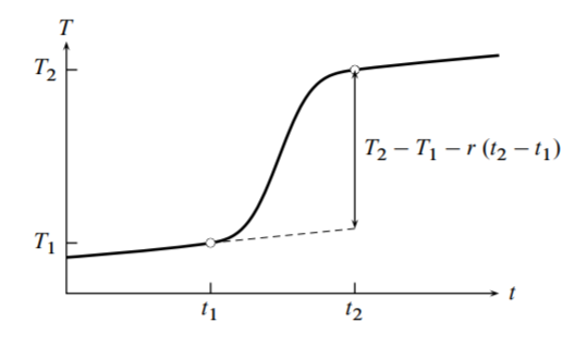
An example of a measured heating curve (temperature \(T\) as a function of time \(t\) ) is shown in Fig. 7.3. We select two points on the heating curve, indicated in the figure by open circles. Time \(t_{1}\) is at or shortly before the instant the heater circuit is closed and electrical heating begins, and time \(t_{2}\) is after the heater circuit has been opened and the slope of the curve has become essentially constant.
In the time periods before \(t_{1}\) and after \(t_{2}\), the temperature may exhibit a slow rate of increase due to the continuous work \(w_{\text {cont }}\) from stirring and temperature measurement. If this work is performed at a constant rate throughout the course of the experiment, the slope is constant and the same in both time periods as shown in the figure.
The relation between the slope and the rate of work is given by a quantity called the energy equivalent, \(\epsilon\). The energy equivalent is the heat capacity of the calorimeter under the conditions of an experiment. The heat capacity of a constant-volume calorimeter is given by \(\epsilon=(\partial U / \partial T)_{V}\) (Eq. 5.6.1). Thus, at times before \(t_{1}\) or after \(t_{2}\), when đ \(w_{\text {el }}\) is zero and \(\mathrm{d} U\) equals \(w_{\text {cont }}\), the slope \(r\) of the heating curve is given by
\[
r=\frac{\mathrm{d} T}{\mathrm{~d} t}=\frac{\mathrm{d} T}{\mathrm{~d} U} \frac{\mathrm{d} U}{\mathrm{~d} t}=\frac{1}{\epsilon} \frac{\mathrm{d} w_{\text {cont }}}{\mathrm{d} t}
\]
The rate of the continuous work is therefore \(\mathrm{d} w_{\text {cont }} / \mathrm{d} t=\epsilon r\). This rate is constant throughout the experiment. In the time interval from \(t_{1}\) to \(t_{2}\), the total quantity of continuous work is \(w_{\text {cont }}=\epsilon r\left(t_{2}-t_{1}\right)\), where \(r\) is the slope of the heating curve measured outside this time interval.
To find the energy equivalent, we integrate Eq. \(7.3 .13\) between the two points on the curve:
\[
\Delta U=w_{\mathrm{el}}+w_{\mathrm{cont}}=w_{\mathrm{el}}+\epsilon r\left(t_{2}-t_{1}\right)
\] (constant \(V\) )
Then the average heat capacity between temperatures \(T_{1}\) and \(T_{2}\) is
\[
\epsilon=\frac{\Delta U}{T_{2}-T_{1}}=\frac{w_{\mathrm{el}}+\epsilon r\left(t_{2}-t_{1}\right)}{T_{2}-T_{1}}
\]
Solving for \(\epsilon\), we obtain
\[
\epsilon=\frac{w_{\mathrm{el}}}{T_{2}-T_{1}-r\left(t_{2}-t_{1}\right)}
\]
The value of the denominator on the right side is indicated by the vertical line in Fig. 7.3. It is the temperature change that would have been observed if the same quantity of electrical work had been performed without the continuous work.
Next, consider the heating process in a calorimeter at constant pressure. In this case the enthalpy change is given by \(\mathrm{d} H=\mathrm{d} U+p \mathrm{~d} V\) which, with substitution from Eq. 7.3.12, becomes
\[
\mathrm{d} H=\mathrm{d} w_{\mathrm{el}}+\mathrm{d} w_{\mathrm{cont}}
\]
(constant \(p\) )
We follow the same procedure as for the constant-volume calorimeter, using Eq. \(7.3 .18\) in place of Eq. \(7.3 .13\) and equating the energy equivalent \(\epsilon\) to \((\partial H / \partial T)_{p}\), the heat capacity of the calorimeter at constant pressure (Eq. 5.6.3). We obtain the relation
\[
\Delta H=w_{\mathrm{el}}+w_{\mathrm{cont}}=w_{\mathrm{el}}+\epsilon r\left(t_{2}-t_{1}\right)
\]
(constant \(p\) )
in place of Eq. \(7.3 .15\) and end up again with the expression of Eq. \(7.3 .17\) for \(\epsilon\).
The value of \(\epsilon\) calculated from Eq. \(7.3 .17\) is an average value for the temperature interval from \(T_{1}\) to \(T_{2}\), and we can identify this value with the heat capacity at the temperature of the midpoint of the interval. By taking the difference of values of \(\epsilon\) measured with and without the phase of interest present in the calorimeter, we obtain \(C_{V}\) or \(C_{p}\) for the phase alone.
It may seem paradoxical that we can use an adiabatic process, one without heat, to evaluate a quantity defined by heat (heat capacity \(=\mathrm{d} q / \mathrm{d} T\) ). The explanation is that energy transferred into the adiabatic calorimeter as electrical work, and dissipated completely to thermal energy, substitutes for the heat that would be needed for the same change of state without electrical work.
Isothermal-jacket calorimeters
A second common type of calorimeter is similar in construction to an adiabatic calorimeter, except that the surrounding jacket is maintained at constant temperature. It is sometimes called an isoperibol calorimeter. A correction is made for heat transfer resulting from the difference in temperature across the gap separating the jacket from the outer surface of the calorimeter. It is important in making this correction that the outer surface have a uniform temperature without "hot spots."
Assume the outer surface of the calorimeter has a uniform temperature \(T\) that varies with time, the jacket temperature has a constant value \(T_{\text {ext }}\), and convection has been eliminated by evacuating the gap. Then heat transfer is by conduction and radiation, and its rate
is given by Newton's law of cooling
\[
\frac{\mathrm{d} q}{\mathrm{~d} t}=-k\left(T-T_{\mathrm{ext}}\right)
\]
where \(k\) is a constant (the thermal conductance). Heat flows from a warmer to a cooler body, so đ \(q / \mathrm{d} t\) is positive if \(T\) is less than \(T_{\text {ext }}\) and negative if \(T\) is greater than \(T_{\text {ext }}\).
The possible kinds of work are the same as for the adiabatic calorimeter: expansion work \(-p \mathrm{~d} V\), intermittent work \(w_{\mathrm{el}}\) done by the heater circuit, and continuous work \(w_{\text {cont }}\). By combining the first law and Eq. 7.3.20, we obtain the following relation for the rate at which the internal energy changes:
\[
\frac{\mathrm{d} U}{\mathrm{~d} t}=\frac{\mathrm{d} q}{\mathrm{~d} t}+\frac{\mathrm{d} w}{\mathrm{~d} t}=-k\left(T-T_{\mathrm{ext}}\right)-p \frac{\mathrm{d} V}{\mathrm{~d} t}+\frac{\mathrm{d} w_{\mathrm{el}}}{\mathrm{d} t}+\frac{\mathrm{d} w_{\text {cont }}}{\mathrm{d} t}
\]
For heating at constant volume \((\mathrm{d} V / \mathrm{d} t=0)\), this relation becomes
\[
\frac{\mathrm{d} U}{\mathrm{~d} t}=-k\left(T-T_{\mathrm{ext}}\right)+\frac{\mathrm{d} w_{\mathrm{el}}}{\mathrm{d} t}+\frac{\mathrm{d} w_{\mathrm{cont}}}{\mathrm{d} t}
\](constant \(V\) )
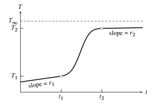
An example of a heating curve is shown in Fig. 7.4. In contrast to the curve of Fig. \(7.3\), the slopes are different before and after the heating interval due to changed rate of heat flow. Times \(t_{1}\) and \(t_{2}\) are before and after the heater circuit is closed. In any time interval before time \(t_{1}\) or after time \(t_{2}\), the system behaves as if it is approaching a steady state of constant temperature \(T_{\infty}\) (called the convergence temperature), which it would eventually reach if the experiment were continued without closing the heater circuit. \(T_{\infty}\) is greater than \(T_{\text {ext }}\) because of the energy transferred to the system by stirring and electrical temperature measurement. By setting \(\mathrm{d} U / \mathrm{d} t\) and \(\mathrm{d} w_{\mathrm{el}} / \mathrm{d} t\) equal to zero and \(T\) equal to \(T_{\infty}\) in Eq. 7.3.22, we obtain đ \(w_{\text {cont }} / \mathrm{d} t=k\left(T_{\infty}-T_{\text {ext }}\right) .\) We assume d \(w_{\text {cont }} / \mathrm{d} t\) is constant. Substituting this expression into Eq. \(7.3 .22\) gives us a general expression for the rate at which \(U\) changes in terms of the unknown quantities \(k\) and \(T_{\infty}\) :
\[
\frac{\mathrm{d} U}{\mathrm{~d} t}=-k\left(T-T_{\infty}\right)+\frac{\mathrm{d} w_{\mathrm{el}}}{\mathrm{d} t}
\]
(constant \(V\) )
This relation is valid throughout the experiment, not only while the heater circuit is closed. If we multiply by \(\mathrm{d} t\) and integrate from \(t_{1}\) to \(t_{2}\), we obtain the internal energy change in the time interval from \(t_{1}\) to \(t_{2}\) :
\[
\Delta U=-k \int_{t_{1}}^{t_{2}}\left(T-T_{\infty}\right) \mathrm{d} t+w_{\mathrm{el}}
\]
(constant \(V\) )
All the intermittent work \(w_{\mathrm{el}}\) is performed in this time interval.
The derivation of Eq. \(7.3 .24\) is a general one. The equation can be applied also to a isothermal-jacket calorimeter in which a reaction is occurring. Section \(11.5 .2\) will mention the use of this equation for an internal energy correction of a reaction calorimeter with an isothermal jacket.
The average value of the energy equivalent in the temperature range \(T_{1}\) to \(T_{2}\) is
\[
\epsilon=\frac{\Delta U}{T_{2}-T_{1}}=\frac{-\epsilon(k / \epsilon) \int_{t_{1}}^{t_{2}}\left(T-T_{\infty}\right) \mathrm{d} t+w_{\mathrm{el}}}{T_{2}-T_{1}}
\]
Solving for \(\epsilon\), we obtain
\[
\epsilon=\frac{w_{\mathrm{el}}}{\left(T_{2}-T_{1}\right)+(k / \epsilon) \int_{t_{1}}^{t_{2}}\left(T-T_{\infty}\right) \mathrm{d} t}
\]
The value of \(w_{\mathrm{el}}\) is known from \(w_{\mathrm{el}}=I^{2} R_{\mathrm{el}} \Delta t\), where \(\Delta t\) is the time interval during which the heater circuit is closed. The integral can be evaluated numerically once \(T_{\infty}\) is known.
For heating at constant pressure, \(\mathrm{d} H\) is equal to \(\mathrm{d} U+p \mathrm{~d} V\), and we can write
\[
\frac{\mathrm{d} H}{\mathrm{~d} t}=\frac{\mathrm{d} U}{\mathrm{~d} t}+p \frac{\mathrm{d} V}{\mathrm{~d} t}=-k\left(T-T_{\mathrm{ext}}\right)+\frac{\mathrm{d} w_{\mathrm{el}}}{\mathrm{d} t}+\frac{\mathrm{d} w_{\mathrm{cont}}}{\mathrm{d} t}
\]
(constant \(p\) )
which is analogous to Eq. 7.3.22. By the procedure described above for the case of constant \(V\), we obtain
\[
\Delta H=-k \int_{t_{1}}^{t_{2}}\left(T-T_{\infty}\right) \mathrm{d} t+w_{\mathrm{el}}
\]
(constant \(p\) )
At constant \(p\), the energy equivalent is equal to \(C_{p}=\Delta H /\left(T_{2}-T_{1}\right)\), and the final expression for \(\epsilon\) is the same as that given by Eq. 7.3.26.
To obtain values of \(k / \epsilon\) and \(T_{\infty}\) for use in Eq. 7.3.26, we need the slopes of the heating curve in time intervals (rating periods) just before \(t_{1}\) and just after \(t_{2}\). Consider the case of constant volume. In these intervals, \(\mathrm{d} w_{\mathrm{el}} / \mathrm{d} t\) is zero and \(\mathrm{d} U / \mathrm{d} t\) equals \(-k\left(T-T_{\infty}\right)\) (from Eq. 7.3.23). The heat capacity at constant volume is \(C_{V}=\mathrm{d} U / \mathrm{d} T\). The slope \(r\) in general is then given by
\[
r=\frac{\mathrm{d} T}{\mathrm{~d} t}=\frac{\mathrm{d} T}{\mathrm{~d} U} \frac{\mathrm{d} U}{\mathrm{~d} t}=-(k / \epsilon)\left(T-T_{\infty}\right)
\]
Applying this relation to the points at times \(t_{1}\) and \(t_{2}\), we have the following simultaneous equations in the unknowns \(k / \epsilon\) and \(T_{\infty}\) :
\[
r_{1}=-(k / \epsilon)\left(T_{1}-T_{\infty}\right) \quad r_{2}=-(k / \epsilon)\left(T_{2}-T_{\infty}\right)
\]
The solutions are
\[
(k / \epsilon)=\frac{r_{1}-r_{2}}{T_{2}-T_{1}} \quad T_{\infty}=\frac{r_{1} T_{2}-r_{2} T_{1}}{r_{1}-r_{2}}
\]
Finally, \(k\) is given by
\[
k=(k / \epsilon) \epsilon=\left(\frac{r_{1}-r_{2}}{T_{2}-T_{1}}\right) \epsilon
\]
When the pressure is constant, this procedure yields the same relations for \(k / \epsilon, T_{\infty}\), and \(k .\)
Continuous-flow calorimeters
A flow calorimeter is a third type of calorimeter used to measure the heat capacity of a fluid phase. The gas or liquid flows through a tube at a known constant rate past an electrical heater of known constant power input. After a steady state has been achieved in the tube, the temperature increase \(\Del T\) at the heater is measured.
If \(\dw\el/\dt\) is the rate at which electrical work is performed (the electric power) and \(\dif m/\dt\) is the mass flow rate, then in time interval \(\Del t\) a quantity \(w=(\dw\el/\dt)\Del t\) of work is performed on an amount \(n=(\dif m/\dt)\Del t/M\) of the fluid (where \(M\) is the molar mass). If heat flow is negligible, the molar heat capacity of the substance is given by \begin{equation} \Cpm = \frac{w}{n\Del T} = \frac{M(\dw\el/\dt)}{\Del T(\dif m/\dt)} \tag{7.3.33} \end{equation} To correct for the effects of heat flow, \(\Del T\) is usually measured over a range of flow rates and the results extrapolated to infinite flow rate.
7.3.3 Typical values
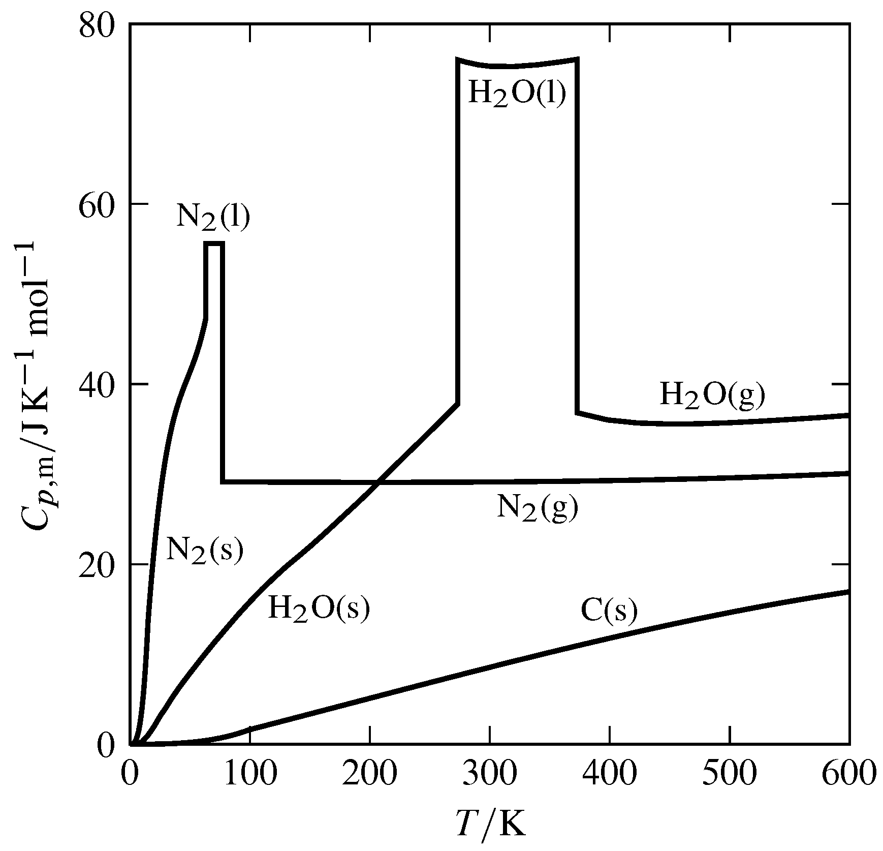
Figure 7.5 Temperature dependence of molar heat capacity at constant pressure (\(p=1\br\)) of H\(_2\)O, N\(_2\), and C(graphite).
Figure 7.5 shows the temperature dependence of \(\Cpm\) for several substances. The discontinuities seen at certain temperatures occur at equilibrium phase transitions. At these temperatures the heat capacity is in effect infinite, since the phase transition of a pure substance involves finite heat with zero temperature change.