
4.4: Derivation of the Mathematical Statement of the Second Law
- Page ID
- 20664

\( \newcommand{\vecs}[1]{\overset { \scriptstyle \rightharpoonup} {\mathbf{#1}} } \)
\( \newcommand{\vecd}[1]{\overset{-\!-\!\rightharpoonup}{\vphantom{a}\smash {#1}}} \)
\( \newcommand{\id}{\mathrm{id}}\) \( \newcommand{\Span}{\mathrm{span}}\)
( \newcommand{\kernel}{\mathrm{null}\,}\) \( \newcommand{\range}{\mathrm{range}\,}\)
\( \newcommand{\RealPart}{\mathrm{Re}}\) \( \newcommand{\ImaginaryPart}{\mathrm{Im}}\)
\( \newcommand{\Argument}{\mathrm{Arg}}\) \( \newcommand{\norm}[1]{\| #1 \|}\)
\( \newcommand{\inner}[2]{\langle #1, #2 \rangle}\)
\( \newcommand{\Span}{\mathrm{span}}\)
\( \newcommand{\id}{\mathrm{id}}\)
\( \newcommand{\Span}{\mathrm{span}}\)
\( \newcommand{\kernel}{\mathrm{null}\,}\)
\( \newcommand{\range}{\mathrm{range}\,}\)
\( \newcommand{\RealPart}{\mathrm{Re}}\)
\( \newcommand{\ImaginaryPart}{\mathrm{Im}}\)
\( \newcommand{\Argument}{\mathrm{Arg}}\)
\( \newcommand{\norm}[1]{\| #1 \|}\)
\( \newcommand{\inner}[2]{\langle #1, #2 \rangle}\)
\( \newcommand{\Span}{\mathrm{span}}\) \( \newcommand{\AA}{\unicode[.8,0]{x212B}}\)
\( \newcommand{\vectorA}[1]{\vec{#1}} % arrow\)
\( \newcommand{\vectorAt}[1]{\vec{\text{#1}}} % arrow\)
\( \newcommand{\vectorB}[1]{\overset { \scriptstyle \rightharpoonup} {\mathbf{#1}} } \)
\( \newcommand{\vectorC}[1]{\textbf{#1}} \)
\( \newcommand{\vectorD}[1]{\overrightarrow{#1}} \)
\( \newcommand{\vectorDt}[1]{\overrightarrow{\text{#1}}} \)
\( \newcommand{\vectE}[1]{\overset{-\!-\!\rightharpoonup}{\vphantom{a}\smash{\mathbf {#1}}}} \)
\( \newcommand{\vecs}[1]{\overset { \scriptstyle \rightharpoonup} {\mathbf{#1}} } \)
\( \newcommand{\vecd}[1]{\overset{-\!-\!\rightharpoonup}{\vphantom{a}\smash {#1}}} \)
\(\newcommand{\avec}{\mathbf a}\) \(\newcommand{\bvec}{\mathbf b}\) \(\newcommand{\cvec}{\mathbf c}\) \(\newcommand{\dvec}{\mathbf d}\) \(\newcommand{\dtil}{\widetilde{\mathbf d}}\) \(\newcommand{\evec}{\mathbf e}\) \(\newcommand{\fvec}{\mathbf f}\) \(\newcommand{\nvec}{\mathbf n}\) \(\newcommand{\pvec}{\mathbf p}\) \(\newcommand{\qvec}{\mathbf q}\) \(\newcommand{\svec}{\mathbf s}\) \(\newcommand{\tvec}{\mathbf t}\) \(\newcommand{\uvec}{\mathbf u}\) \(\newcommand{\vvec}{\mathbf v}\) \(\newcommand{\wvec}{\mathbf w}\) \(\newcommand{\xvec}{\mathbf x}\) \(\newcommand{\yvec}{\mathbf y}\) \(\newcommand{\zvec}{\mathbf z}\) \(\newcommand{\rvec}{\mathbf r}\) \(\newcommand{\mvec}{\mathbf m}\) \(\newcommand{\zerovec}{\mathbf 0}\) \(\newcommand{\onevec}{\mathbf 1}\) \(\newcommand{\real}{\mathbb R}\) \(\newcommand{\twovec}[2]{\left[\begin{array}{r}#1 \\ #2 \end{array}\right]}\) \(\newcommand{\ctwovec}[2]{\left[\begin{array}{c}#1 \\ #2 \end{array}\right]}\) \(\newcommand{\threevec}[3]{\left[\begin{array}{r}#1 \\ #2 \\ #3 \end{array}\right]}\) \(\newcommand{\cthreevec}[3]{\left[\begin{array}{c}#1 \\ #2 \\ #3 \end{array}\right]}\) \(\newcommand{\fourvec}[4]{\left[\begin{array}{r}#1 \\ #2 \\ #3 \\ #4 \end{array}\right]}\) \(\newcommand{\cfourvec}[4]{\left[\begin{array}{c}#1 \\ #2 \\ #3 \\ #4 \end{array}\right]}\) \(\newcommand{\fivevec}[5]{\left[\begin{array}{r}#1 \\ #2 \\ #3 \\ #4 \\ #5 \\ \end{array}\right]}\) \(\newcommand{\cfivevec}[5]{\left[\begin{array}{c}#1 \\ #2 \\ #3 \\ #4 \\ #5 \\ \end{array}\right]}\) \(\newcommand{\mattwo}[4]{\left[\begin{array}{rr}#1 \amp #2 \\ #3 \amp #4 \\ \end{array}\right]}\) \(\newcommand{\laspan}[1]{\text{Span}\{#1\}}\) \(\newcommand{\bcal}{\cal B}\) \(\newcommand{\ccal}{\cal C}\) \(\newcommand{\scal}{\cal S}\) \(\newcommand{\wcal}{\cal W}\) \(\newcommand{\ecal}{\cal E}\) \(\newcommand{\coords}[2]{\left\{#1\right\}_{#2}}\) \(\newcommand{\gray}[1]{\color{gray}{#1}}\) \(\newcommand{\lgray}[1]{\color{lightgray}{#1}}\) \(\newcommand{\rank}{\operatorname{rank}}\) \(\newcommand{\row}{\text{Row}}\) \(\newcommand{\col}{\text{Col}}\) \(\renewcommand{\row}{\text{Row}}\) \(\newcommand{\nul}{\text{Nul}}\) \(\newcommand{\var}{\text{Var}}\) \(\newcommand{\corr}{\text{corr}}\) \(\newcommand{\len}[1]{\left|#1\right|}\) \(\newcommand{\bbar}{\overline{\bvec}}\) \(\newcommand{\bhat}{\widehat{\bvec}}\) \(\newcommand{\bperp}{\bvec^\perp}\) \(\newcommand{\xhat}{\widehat{\xvec}}\) \(\newcommand{\vhat}{\widehat{\vvec}}\) \(\newcommand{\uhat}{\widehat{\uvec}}\) \(\newcommand{\what}{\widehat{\wvec}}\) \(\newcommand{\Sighat}{\widehat{\Sigma}}\) \(\newcommand{\lt}{<}\) \(\newcommand{\gt}{>}\) \(\newcommand{\amp}{&}\) \(\definecolor{fillinmathshade}{gray}{0.9}\)
\( \newcommand{\tx}[1]{\text{#1}} % text in math mode\)
\( \newcommand{\subs}[1]{_{\text{#1}}} % subscript text\)
\( \newcommand{\sups}[1]{^{\text{#1}}} % superscript text\)
\( \newcommand{\st}{^\circ} % standard state symbol\)
\( \newcommand{\id}{^{\text{id}}} % ideal\)
\( \newcommand{\rf}{^{\text{ref}}} % reference state\)
\( \newcommand{\units}[1]{\mbox{$\thinspace$#1}}\)
\( \newcommand{\K}{\units{K}} % kelvins\)
\( \newcommand{\degC}{^\circ\text{C}} % degrees Celsius\)
\( \newcommand{\br}{\units{bar}} % bar (\bar is already defined)\)
\( \newcommand{\Pa}{\units{Pa}}\)
\( \newcommand{\mol}{\units{mol}} % mole\)
\( \newcommand{\V}{\units{V}} % volts\)
\( \newcommand{\timesten}[1]{\mbox{$\,\times\,10^{#1}$}}\)
\( \newcommand{\per}{^{-1}} % minus one power\)
\( \newcommand{\m}{_{\text{m}}} % subscript m for molar quantity\)
\( \newcommand{\CVm}{C_{V,\text{m}}} % molar heat capacity at const.V\)
\( \newcommand{\Cpm}{C_{p,\text{m}}} % molar heat capacity at const.p\)
\( \newcommand{\kT}{\kappa_T} % isothermal compressibility\)
\( \newcommand{\A}{_{\text{A}}} % subscript A for solvent or state A\)
\( \newcommand{\B}{_{\text{B}}} % subscript B for solute or state B\)
\( \newcommand{\bd}{_{\text{b}}} % subscript b for boundary or boiling point\)
\( \newcommand{\C}{_{\text{C}}} % subscript C\)
\( \newcommand{\f}{_{\text{f}}} % subscript f for freezing point\)
\( \newcommand{\mA}{_{\text{m},\text{A}}} % subscript m,A (m=molar)\)
\( \newcommand{\mB}{_{\text{m},\text{B}}} % subscript m,B (m=molar)\)
\( \newcommand{\mi}{_{\text{m},i}} % subscript m,i (m=molar)\)
\( \newcommand{\fA}{_{\text{f},\text{A}}} % subscript f,A (for fr. pt.)\)
\( \newcommand{\fB}{_{\text{f},\text{B}}} % subscript f,B (for fr. pt.)\)
\( \newcommand{\xbB}{_{x,\text{B}}} % x basis, B\)
\( \newcommand{\xbC}{_{x,\text{C}}} % x basis, C\)
\( \newcommand{\cbB}{_{c,\text{B}}} % c basis, B\)
\( \newcommand{\mbB}{_{m,\text{B}}} % m basis, B\)
\( \newcommand{\kHi}{k_{\text{H},i}} % Henry's law constant, x basis, i\)
\( \newcommand{\kHB}{k_{\text{H,B}}} % Henry's law constant, x basis, B\)
\( \newcommand{\arrow}{\,\rightarrow\,} % right arrow with extra spaces\)
\( \newcommand{\arrows}{\,\rightleftharpoons\,} % double arrows with extra spaces\)
\( \newcommand{\ra}{\rightarrow} % right arrow (can be used in text mode)\)
\( \newcommand{\eq}{\subs{eq}} % equilibrium state\)
\( \newcommand{\onehalf}{\textstyle\frac{1}{2}\D} % small 1/2 for display equation\)
\( \newcommand{\sys}{\subs{sys}} % system property\)
\( \newcommand{\sur}{\sups{sur}} % surroundings\)
\( \renewcommand{\in}{\sups{int}} % internal\)
\( \newcommand{\lab}{\subs{lab}} % lab frame\)
\( \newcommand{\cm}{\subs{cm}} % center of mass\)
\( \newcommand{\rev}{\subs{rev}} % reversible\)
\( \newcommand{\irr}{\subs{irr}} % irreversible\)
\( \newcommand{\fric}{\subs{fric}} % friction\)
\( \newcommand{\diss}{\subs{diss}} % dissipation\)
\( \newcommand{\el}{\subs{el}} % electrical\)
\( \newcommand{\cell}{\subs{cell}} % cell\)
\( \newcommand{\As}{A\subs{s}} % surface area\)
\( \newcommand{\E}{^\mathsf{E}} % excess quantity (superscript)\)
\( \newcommand{\allni}{\{n_i \}} % set of all n_i\)
\( \newcommand{\sol}{\hspace{-.1em}\tx{(sol)}}\)
\( \newcommand{\solmB}{\tx{(sol,$\,$$m\B$)}}\)
\( \newcommand{\dil}{\tx{(dil)}}\)
\( \newcommand{\sln}{\tx{(sln)}}\)
\( \newcommand{\mix}{\tx{(mix)}}\)
\( \newcommand{\rxn}{\tx{(rxn)}}\)
\( \newcommand{\expt}{\tx{(expt)}}\)
\( \newcommand{\solid}{\tx{(s)}}\)
\( \newcommand{\liquid}{\tx{(l)}}\)
\( \newcommand{\gas}{\tx{(g)}}\)
\( \newcommand{\pha}{\alpha} % phase alpha\)
\( \newcommand{\phb}{\beta} % phase beta\)
\( \newcommand{\phg}{\gamma} % phase gamma\)
\( \newcommand{\aph}{^{\alpha}} % alpha phase superscript\)
\( \newcommand{\bph}{^{\beta}} % beta phase superscript\)
\( \newcommand{\gph}{^{\gamma}} % gamma phase superscript\)
\( \newcommand{\aphp}{^{\alpha'}} % alpha prime phase superscript\)
\( \newcommand{\bphp}{^{\beta'}} % beta prime phase superscript\)
\( \newcommand{\gphp}{^{\gamma'}} % gamma prime phase superscript\)
\( \newcommand{\apht}{\small\aph} % alpha phase tiny superscript\)
\( \newcommand{\bpht}{\small\bph} % beta phase tiny superscript\)
\( \newcommand{\gpht}{\small\gph} % gamma phase tiny superscript\)
\( \newcommand{\upOmega}{\Omega}\)
\( \newcommand{\dif}{\mathop{}\!\mathrm{d}} % roman d in math mode, preceded by space\)
\( \newcommand{\Dif}{\mathop{}\!\mathrm{D}} % roman D in math mode, preceded by space\)
\( \newcommand{\df}{\dif\hspace{0.05em} f} % df\)
\(\newcommand{\dBar}{\mathop{}\!\mathrm{d}\hspace-.3em\raise1.05ex{\Rule{.8ex}{.125ex}{0ex}}} % inexact differential \)
\( \newcommand{\dq}{\dBar q} % heat differential\)
\( \newcommand{\dw}{\dBar w} % work differential\)
\( \newcommand{\dQ}{\dBar Q} % infinitesimal charge\)
\( \newcommand{\dx}{\dif\hspace{0.05em} x} % dx\)
\( \newcommand{\dt}{\dif\hspace{0.05em} t} % dt\)
\( \newcommand{\difp}{\dif\hspace{0.05em} p} % dp\)
\( \newcommand{\Del}{\Delta}\)
\( \newcommand{\Delsub}[1]{\Delta_{\text{#1}}}\)
\( \newcommand{\pd}[3]{(\partial #1 / \partial #2 )_{#3}} % \pd{}{}{} - partial derivative, one line\)
\( \newcommand{\Pd}[3]{\left( \dfrac {\partial #1} {\partial #2}\right)_{#3}} % Pd{}{}{} - Partial derivative, built-up\)
\( \newcommand{\bpd}[3]{[ \partial #1 / \partial #2 ]_{#3}}\)
\( \newcommand{\bPd}[3]{\left[ \dfrac {\partial #1} {\partial #2}\right]_{#3}}\)
\( \newcommand{\dotprod}{\small\bullet}\)
\( \newcommand{\fug}{f} % fugacity\)
\( \newcommand{\g}{\gamma} % solute activity coefficient, or gamma in general\)
\( \newcommand{\G}{\varGamma} % activity coefficient of a reference state (pressure factor)\)
\( \newcommand{\ecp}{\widetilde{\mu}} % electrochemical or total potential\)
\( \newcommand{\Eeq}{E\subs{cell, eq}} % equilibrium cell potential\)
\( \newcommand{\Ej}{E\subs{j}} % liquid junction potential\)
\( \newcommand{\mue}{\mu\subs{e}} % electron chemical potential\)
\( \newcommand{\defn}{\,\stackrel{\mathrm{def}}{=}\,} % "equal by definition" symbol\)
\( \newcommand{\D}{\displaystyle} % for a line in built-up\)
\( \newcommand{\s}{\smash[b]} % use in equations with conditions of validity\)
\( \newcommand{\cond}[1]{\\[-2.5pt]{}\tag*{#1}}\)
\( \newcommand{\nextcond}[1]{\\[-5pt]{}\tag*{#1}}\)
\( \newcommand{\R}{8.3145\units{J$\,$K$\per\,$mol$\per$}} % gas constant value\)
\( \newcommand{\Rsix}{8.31447\units{J$\,$K$\per\,$mol$\per$}} % gas constant value - 6 sig figs\)
\( \newcommand{\jn}{\hspace3pt\lower.3ex{\Rule{.6pt}{2ex}{0ex}}\hspace3pt} \)
\( \newcommand{\ljn}{\hspace3pt\lower.3ex{\Rule{.6pt}{.5ex}{0ex}}\hspace-.6pt\raise.45ex{\Rule{.6pt}{.5ex}{0ex}}\hspace-.6pt\raise1.2ex{\Rule{.6pt}{.5ex}{0ex}} \hspace3pt} \)
\( \newcommand{\lljn}{\hspace3pt\lower.3ex{\Rule{.6pt}{.5ex}{0ex}}\hspace-.6pt\raise.45ex{\Rule{.6pt}{.5ex}{0ex}}\hspace-.6pt\raise1.2ex{\Rule{.6pt}{.5ex}{0ex}}\hspace1.4pt\lower.3ex{\Rule{.6pt}{.5ex}{0ex}}\hspace-.6pt\raise.45ex{\Rule{.6pt}{.5ex}{0ex}}\hspace-.6pt\raise1.2ex{\Rule{.6pt}{.5ex}{0ex}}\hspace3pt} \)
4.4.1 The existence of the entropy function
This section derives the existence and properties of the state function called entropy.
Consider an arbitrary cyclic process of a closed system. To avoid confusion, this system will be the “experimental system” and the process will be the “experimental process” or “experimental cycle.” There are no restrictions on the contents of the experimental system—it may have any degree of complexity whatsoever. The experimental process may involve more than one kind of work, phase changes and reactions may occur, there may be temperature and pressure gradients, constraints and external fields may be present, and so on. All parts of the process must be either irreversible or reversible, but not impossible.
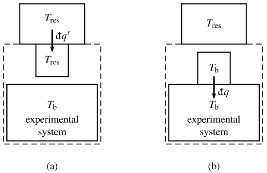
Figure 4.8 Experimental system, Carnot engine (represented by a small square box), and heat reservoir. The dashed lines indicate the boundary of the supersystem.
(a) Reversible heat transfer between heat reservoir and Carnot engine.
(b) Heat transfer between Carnot engine and experimental system.
The infinitesimal quantities \(\dq'\) and \(\dq\) are positive for transfer in the directions indicated by the arrows.
We imagine that the experimental cycle is carried out in a special way that allows us to apply the Kelvin–Planck statement of the second law. The heat transferred across the boundary of the experimental system in each infinitesimal path element of the cycle is exchanged with a hypothetical Carnot engine. The combination of the experimental system and the Carnot engine is a closed supersystem (see Fig. 4.8). In the surroundings of the supersystem is a heat reservoir of arbitrary constant temperature \(T\subs{res}\). By allowing the supersystem to exchange heat with only this single heat reservoir, we will be able to apply the Kelvin–Planck statement to a cycle of the supersystem.
This procedure is similar to ones described by A. B. Pippard (Elements of Classical Thermodynamics for Advanced Students of Physics, Cambridge University Press, Cambridge, 1966, Chap. 4); C. J. Adkins (Equilibrium Thermodynamics, 3rd edition, Cambridge University Press, Cambridge, 1983, Chap. 5); and Peter T. Landsberg (Thermodynamics and Statistical Mechanics, Dover Publications, Inc., New York, 1990, p. 53).
We assume that we are able to control changes of the work coordinates of the experimental system from the surroundings of the supersystem. We are also able to control the Carnot engine from these surroundings, for example by moving the piston of a cylinder-and-piston device containing the working substance. Thus the energy transferred by work across the boundary of the experimental system, and the work required to operate the Carnot engine, is exchanged with the surroundings of the supersystem.
During each stage of the experimental process with nonzero heat, we allow the Carnot engine to undergo many infinitesimal Carnot cycles with infinitesimal quantities of heat and work. In one of the isothermal steps of each Carnot cycle, the Carnot engine is in thermal contact with the heat reservoir, as depicted in Fig. 4.8(a). In this step the Carnot engine has the same temperature as the heat reservoir, and reversibly exchanges heat \(\dq'\) with it. The sign convention is that \(\dq'\) is positive if heat is transferred in the direction of the arrow, from the heat reservoir to the Carnot engine.
In the other isothermal step of the Carnot cycle, the Carnot engine is in thermal contact with the experimental system at a portion of the system’s boundary. as depicted in Fig. 4.8(b). The Carnot engine now has the same temperature, \(T\bd\), as the experimental system at this part of the boundary, and exchanges heat with it. The heat \(\dq\) is positive if the transfer is into the experimental system.
The relation between temperatures and heats in the isothermal steps of a Carnot cycle is given by Eq. 4.3.15. From this relation we obtain, for one infinitesimal Carnot cycle, the relation \(T\bd/T\subs{res}=\dq/\dq'\), or \begin{equation} \dq'=T\subs{res}\frac{\dq}{T\bd} \tag{4.4.1} \end{equation}
After many infinitesimal Carnot cycles, the experimental cycle is complete, the experimental system has returned to its initial state, and the Carnot engine has returned to its initial state in thermal contact with the heat reservoir. Integration of Eq. 4.4.1 around the experimental cycle gives the net heat entering the supersystem during the process: \begin{gather} q'=T\subs{res} \tag{4.4.2} \oint\!\frac{\dq}{T\bd} \end{gather} The integration here is over each path element of the experimental process and over each surface element of the boundary of the experimental system.
Keep in mind that the value of the cyclic integral \(\oint\dq/T\bd\) depends only on the path of the experimental cycle, that this process can be reversible or irreversible, and that \(T\subs{res}\) is a positive constant.
In this experimental cycle, could the net heat \(q'\) transferred to the supersystem be positive? If so, the net work would be negative (to make the internal energy change zero) and the supersystem would have converted heat from a single heat reservoir completely into work, a process the Kelvin–Planck statement of the second law says is impossible. Therefore it is impossible for \(q'\) to be positive, and from Eq. 4.4.2 we obtain the relation \begin{gather} \s{\oint\!\frac{\dq}{T\bd}\leq 0} \tag{4.4.3} \cond{(cyclic process of a closed system)} \end{gather} This relation is known as the Clausius inequality. It is valid only if the integration is taken around a cyclic path in a direction with nothing but reversible and irreversible changes—the path must not include an impossible change, such as the reverse of an irreversible change. The Clausius inequality says that if a cyclic path meets this specification, it is impossible for the cyclic integral \(\oint(\dq/T\bd)\) to be positive.
If the entire experimental cycle is adiabatic (which is only possible if the process is reversible), the Carnot engine is not needed and Eq. 4.4.3 can be replaced by \(\oint(\dq/T\bd)=0\).
Next let us investigate a reversible nonadiabatic process of the closed experimental system. Starting with a particular equilibrium state A, we carry out a reversible process in which there is a net flow of heat into the system, and in which \(\dq\) is either positive or zero in each path element. The final state of this process is equilibrium state B. If each infinitesimal quantity of heat \(\dq\) is positive or zero during the process, then the integral \(\int_{\tx{A}}^{\tx{B}}(\dq/T\bd)\) must be positive. In this case the Clausius inequality tells us that if the system completes a cycle by returning from state B back to state A by a different path, the integral \(\int_{\tx{B}}^{\tx{A}}(\dq/T\bd)\) for this second path must be negative. Therefore the change B\(\ra\)A cannot be carried out by any adiabatic process.
Any reversible process can be carried out in reverse. Thus, by reversing the reversible nonadiabatic process, it is possible to change the state from B to A by a reversible process with a net flow of heat out of the system and with \(\dq\) either negative or zero in each element of the reverse path. In contrast, the absence of an adiabatic path from B to A means that it is impossible to carry out the change A\(\ra\)B by a reversible adiabatic process.
The general rule, then, is that whenever equilibrium state A of a closed system can be changed to equilibrium state B by a reversible process with finite “one-way” heat (i.e., the flow of heat is either entirely into the system or else entirely out of it), it is impossible for the system to change from either of these states to the other by a reversible adiabatic process.
A simple example will relate this rule to experience. We can increase the temperature of a liquid by allowing heat to flow reversibly into the liquid. It is impossible to duplicate this change of state by a reversible process without heat—that is, by using some kind of reversible work. The reason is that reversible work involves the change of a work coordinate that brings the system to a different final state. There is nothing in the rule that says we can’t increase the temperature irreversibly without heat, as we can for instance with stirring work.
States A and B can be arbitrarily close. We conclude that every equilibrium state of a closed system has other equilibrium states infinitesimally close to it that are inaccessible by a reversible adiabatic process. This is Carathéodory’s principle of adiabatic inaccessibility. (Constantin Carathéodory in 1909 combined this principle with a mathematical theorem\(—\)Carathéodory’s theorem\(—\)to deduce the existence of the entropy function. The derivation outlined here avoids the complexities of that mathematical treatment and leads to the same results.)
Next let us consider the reversible adiabatic processes that are possible. To carry out a reversible adiabatic process, starting at an initial equilibrium state, we use an adiabatic boundary and slowly vary one or more of the work coordinates. A certain final temperature will result. It is helpful in visualizing this process to think of an \(N\)-dimensional space in which each axis represents one of the \(N\) independent variables needed to describe an equilibrium state. A point in this space represents an equilibrium state, and the path of a reversible process can be represented as a curve in this space.
A suitable set of independent variables for equilibrium states of a closed system of uniform temperature consists of the temperature \(T\) and each of the work coordinates (Sec. 3.10). We can vary the work coordinates independently while keeping the boundary adiabatic, so the paths for possible reversible adiabatic processes can connect any arbitrary combinations of work coordinate values.
There is, however, the additional dimension of temperature in the \(N\)-dimensional space. Do the paths for possible reversible adiabatic processes, starting from a common initial point, lie in a volume in the \(N\)-dimensional space? Or do they fall on a surface described by \(T\) as a function of the work coordinates? If the paths lie in a volume, then every point in a volume element surrounding the initial point must be accessible from the initial point by a reversible adiabatic path. This accessibility is precisely what Carathéodory’s principle of adiabatic inaccessibility denies. Therefore, the paths for all possible reversible adiabatic processes with a common initial state must lie on a unique surface. This is an \((N-1)\)-dimensional hypersurface in the \(N\)-dimensional space, or a curve if \(N\) is \(2\). One of these surfaces or curves will be referred to as a reversible adiabatic surface.
Now consider the initial and final states of a reversible process with one-way heat (i.e., each nonzero infinitesimal quantity of heat \(\dq\) has the same sign). Since we have seen that it is impossible for there to be a reversible adiabatic path between these states, the points for these states must lie on different reversible adiabatic surfaces that do not intersect anywhere in the \(N\)-dimensional space. Consequently, there is an infinite number of nonintersecting reversible adiabatic surfaces filling the \(N\)-dimensional space. (To visualize this for \(N=3\), think of a flexed stack of paper sheets; each sheet represents a different reversible adiabatic surface in three-dimensional space.) A reversible, nonadiabatic process with one-way heat is represented by a path beginning at a point on one reversible adiabatic surface and ending at a point on a different surface. If \(q\) is positive, the final surface lies on one side of the initial surface, and if \(q\) is negative, the final surface is on the opposite side.
4.4.2 Using reversible processes to define the entropy
The existence of reversible adiabatic surfaces is the justification for defining a new state function \(S\), the entropy. \(S\) is specified to have the same value everywhere on one of these surfaces, and a different, unique value on each different surface. In other words, the reversible adiabatic surfaces are surfaces of constant entropy in the \(N\)-dimensional space. The fact that the surfaces fill this space without intersecting ensures that \(S\) is a state function for equilibrium states, because any point in this space represents an equilibrium state and also lies on a single reversible adiabatic surface with a definite value of \(S\).
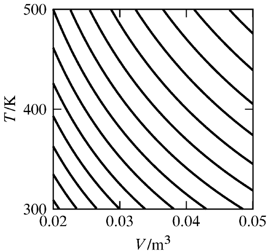
Figure 4.9 A family of reversible adiabatic curves (two-dimensional reversible adiabatic surfaces) for an ideal gas with \(V\) and \(T\) as independent variables. A reversible adiabatic process moves the state of the system along a curve, whereas a reversible process with positive heat moves the state from one curve to another above and to the right. The curves are calculated for \(n = 1\mol\) and \(\CVm = (3/2)R\). Adjacent curves differ in entropy by \(1\units{J K\(^{-1}\)}\).
We know the entropy function must exist, because the reversible adiabatic surfaces exist. For instance, Fig. 4.9 shows a family of these surfaces for a closed system of a pure substance in a single phase. In this system, \(N\) is equal to 2, and the surfaces are two-dimensional curves. Each curve is a contour of constant \(S\). At this stage in the derivation, our assignment of values of \(S\) to the different curves is entirely arbitrary.
How can we assign a unique value of \(S\) to each reversible adiabatic surface? We can order the values by letting a reversible process with positive one-way heat, which moves the point for the state to a new surface, correspond to an increase in the value of \(S\). Negative one-way heat will then correspond to decreasing \(S\). We can assign an arbitrary value to the entropy on one particular reversible adiabatic surface. (The third law of thermodynamics is used for this purpose—see Sec. 6.1.) Then all that is needed to assign a value of \(S\) to each equilibrium state is a formula for evaluating the difference in the entropies of any two surfaces.
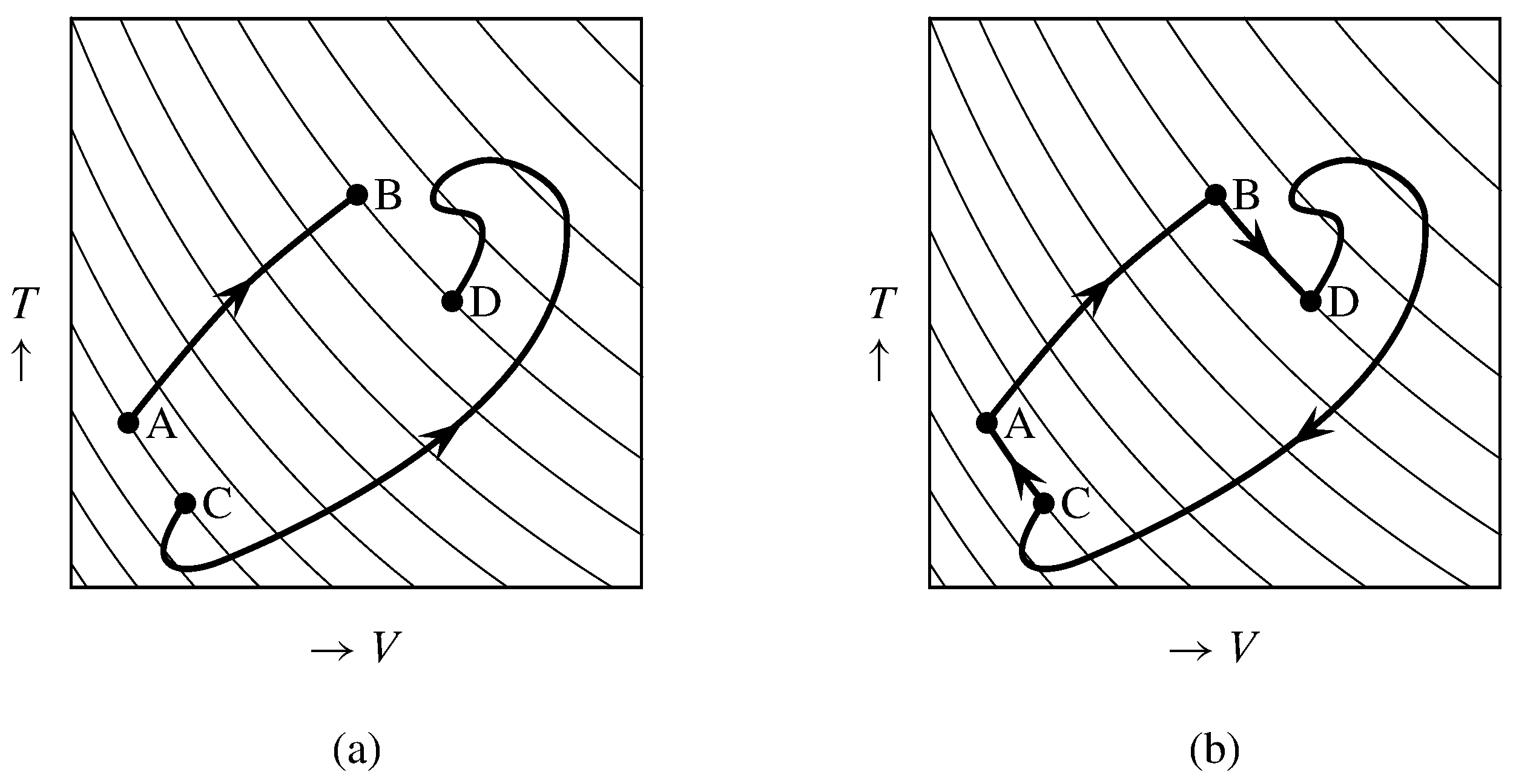
Figure 4.10 Reversible paths in \(V\)–\(T\) space. The thin curves are reversible adiabatic surfaces.
(a) Two paths connecting the same pair of reversible adiabatic surfaces.
(b) A cyclic path.
Consider a reversible process with positive one-way heat that changes the system from state A to state B. The path for this process must move the system from a reversible adiabatic surface of a certain entropy to a different surface of greater entropy. An example is the path A\(\ra\)B in Fig. 4.10(a). (The adiabatic surfaces in this figure are actually two-dimensional curves.) As before, we combine the experimental system with a Carnot engine to form a supersystem that exchanges heat with a single heat reservoir of constant temperature \(T\subs{res}\). The net heat entering the supersystem, found by integrating Eq. 4.4.1, is \begin{equation} q' = T\subs{res} \int_{\tx{A}}^{\tx{B}} \frac{\dq}{T\bd} \tag{4.4.4} \end{equation} and it is positive.
Suppose the same experimental system undergoes a second reversible process, not necessarily with one-way heat, along a different path connecting the same pair of reversible adiabatic surfaces. This could be path C\(\ra\)D in Fig. 4.10(a). The net heat entering the supersystem during this second process is \(q''\): \begin{equation} q'' = T\subs{res} \int_{\tx{C}}^{\tx{D}} \frac{\dq}{T\bd} \tag{4.4.5} \end{equation} We can then devise a cycle of the supersystem in which the experimental system undergoes the reversible path A\(\ra\)B\(\ra\)D\(\ra\)C\(\ra\)A, as shown in Fig. 4.10(b). Step A\(\ra\)B is the first process described above, step D\(\ra\)C is the reverse of the second process described above, and steps B\(\ra\)D and C\(\ra\)A are reversible and adiabatic. The net heat entering the supersystem in the cycle is \(q' - q''\). In the reverse cycle the net heat is \(q''-q'\). In both of these cycles the heat is exchanged with a single heat reservoir; therefore, according to the Kelvin–Planck statement, neither cycle can have positive net heat. Therefore \(q'\) and \(q''\) must be equal, and Eqs. 4.4.4 and 4.4.5 then show the integral \(\int(\dq/T\bd)\) has the same value when evaluated along either of the reversible paths from the lower to the higher entropy surface.
Note that since the second path (C\(\ra\)D) does not necessarily have one-way heat, it can take the experimental system through any sequence of intermediate entropy values, provided it starts at the lower entropy surface and ends at the higher. Furthermore, since the path is reversible, it can be carried out in reverse resulting in reversal of the signs of \(\Del S\) and \(\int(\dq/T\bd)\).
It should now be apparent that a satisfactory formula for defining the entropy change of a reversible process in a closed system is \begin{gather} \s{ \Del S = \int\!\frac{\dq}{T\bd} } \tag{4.4.6} \cond{(reversible process,} \nextcond{closed system)} \end{gather} This formula satisfies the necessary requirements: it makes the value of \(\Del S\) positive if the process has positive one-way heat, negative if the process has negative one-way heat, and zero if the process is adiabatic. It gives the same value of \(\Del S\) for any reversible change between the same two reversible adiabatic surfaces, and it makes the sum of the \(\Del S\) values of several consecutive reversible processes equal to \(\Del S\) for the overall process.
In Eq. 4.4.6, \(\Del S\) is the entropy change when the system changes from one arbitrary equilibrium state to another. If the change is an infinitesimal path element of a reversible process, the equation becomes \begin{gather} \s{ \dif S = \frac{\dq}{T\bd} } \tag{4.4.7} \cond{(reversible process,} \nextcond{closed system)} \end{gather} It is common to see this equation written in the form \(\dif S = \dq\rev/T\), where \(\dq\rev\) denotes an infinitesimal quantity of heat in a reversible process.
In Eq. 4.4.7, the quantity \(1/T\bd\) is called an integrating factor for \(\dq\), a factor that makes the product \((1/T\bd)\dq\) be the infinitesimal change of a state function. The quantity \(c/T\bd\), where \(c\) is any nonzero constant, would also be a satisfactory integrating factor; so the definition of entropy, using \(c{=}1\), is actually one of an infinite number of possible choices for assigning values to the reversible adiabatic surfaces.
4.4.3 Some properties of the entropy
It is not difficult to show that the entropy of a closed system in an equilibrium state is an extensive property. Suppose a system of uniform temperature \(T\) is divided into two closed subsystems A and B. When a reversible infinitesimal change occurs, the entropy changes of the subsystems are \(\dif S\subs{A} = \dq\subs{A}/T\) and \(\dif S\subs{B} = \dq\subs{B}/T\) and of the system \(\dif S = \dq/T\). But \(\dq\) is the sum of \(\dq\subs{A}\) and \(\dq\subs{B}\), which gives \(\dif S = \dif S\subs{A} + \dif S\subs{B}\). Thus, the entropy changes are additive, so that entropy must be extensive: \(S=S\subs{A}+S\subs{B}\). (The argument is not quite complete, because we have not shown that when each subsystem has an entropy of zero, so does the entire system. The zero of entropy will be discussed in Sec. 6.1.)
How can we evaluate the entropy of a particular equilibrium state of the system? We must assign an arbitrary value to one state and then evaluate the entropy change along a reversible path from this state to the state of interest using \(\Del S=\int(\dq/T\bd)\).
We may need to evaluate the entropy of a nonequilibrium state. To do this, we imagine imposing hypothetical internal constraints that change the nonequilibrium state to a constrained equilibrium state with the same internal structure. Some examples of such internal constraints were given in Sec. 2.4.4, and include rigid adiabatic partitions between phases of different temperature and pressure, semipermeable membranes to prevent transfer of certain species between adjacent phases, and inhibitors to prevent chemical reactions.
We assume that we can, in principle, impose or remove such constraints reversibly without heat, so there is no entropy change. If the nonequilibrium state includes macroscopic internal motion, the imposition of internal constraints involves negative reversible work to bring moving regions of the system to rest. This concept amounts to defining the entropy of a state with macroscopic internal motion to be the same as the entropy of a state with the same internal structure but without the motion, i.e., the same state frozen in time. By this definition, \(\Del S\) for a purely mechanical process (Sec. 3.2.3) is zero.
If the system is nonuniform over its extent, the internal constraints will partition it into practically-uniform regions whose entropy is additive. The entropy of the nonequilibrium state is then found from \(\Del S=\int(\dq/T\bd)\) using a reversible path that changes the system from an equilibrium state of known entropy to the constrained equilibrium state with the same entropy as the state of interest. This procedure allows every possible state (at least conceptually) to have a definite value of \(S\).